library(dplyr)
library(ggplot2)
source("../../utils.R")R implementation
In the previous page, we described how to conceptually translate an experimental design into a hierarchy. We now need to rename the variables in the dataset obtained from the experiment to match the GPMelt nomenclature.
The code below is written in R, but you are free to use any language for this step.
1 Prerequisites (Library)
We begin with loading the necessary libraries.
2 Creation of a dummy dataset
For the purpose of the tutorial, we create a dummy dataset corresponding to the dataset modeled in this Video.
In this protein-level TPP-TR experimental design, we have:
- Three conditions (control \(Ctrl\), treatment \(C1\) and treatment \(C2\)).
- The treatment conditions have \(2\) replicates each, while the control condition has \(4\) replicates.
- Each replicate is observed across \(10\) temperatures.
- Additionally, we consider \(3\) proteins: \(P1, P2\) and \(P3\).
set.seed(123)

dummy_dataset <- data.frame(
  protein_ID = rep(c("P1","P2","P3"),each=80),
  treatment = rep(c(rep(c("control"), each = 40), rep(c("treatment_C1", "treatment_C2"), each = 20 )), times=3),
  replicate = rep(c(rep(c(1,2,3,4), each = 10), rep(rep(c(1,2), each = 10), times =2) ), times=3),
  temperature = rep(c(37.0, 40.4, 44.0,46.9,49.8,52.9,55.5,58.6,62.0,66.3), times = 24),
scaled_intensity = abs(rnorm(240))
)

head(dummy_dataset)
protein_ID treatment replicate temperature scaled_intensity
1 P1 control 1 37.0 0.56047565
2 P1 control 1 40.4 0.23017749
3 P1 control 1 44.0 1.55870831
4 P1 control 1 46.9 0.07050839
5 P1 control 1 49.8 0.12928774
6 P1 control 1 52.9 1.71506499Below is a summary of the content of the dataset for each protein_ID:
dummy_dataset %>%
  group_by(protein_ID, treatment, replicate) %>%
  summarise(NumberOfTemperatures = n_distinct(temperature)) %>%
  print(n = nrow(.))
# A tibble: 24 × 4
# Groups: protein_ID, treatment [9]
protein_ID treatment replicate NumberOfTemperatures
<chr> <chr> <dbl> <int>
1 P1 control 1 10
2 P1 control 2 10
3 P1 control 3 10
4 P1 control 4 10
5 P1 treatment_C1 1 10
6 P1 treatment_C1 2 10
7 P1 treatment_C2 1 10
8 P1 treatment_C2 2 10
9 P2 control 1 10
10 P2 control 2 10
11 P2 control 3 10
12 P2 control 4 10
13 P2 treatment_C1 1 10
14 P2 treatment_C1 2 10
15 P2 treatment_C2 1 10
16 P2 treatment_C2 2 10
17 P3 control 1 10
18 P3 control 2 10
19 P3 control 3 10
20 P3 control 4 10
21 P3 treatment_C1 1 10
22 P3 treatment_C1 2 10
23 P3 treatment_C2 1 10
24 P3 treatment_C2 2 103 Renaming the variables
In the Video, the experimental design with replicates and conditions for each ID is translated into a three-level hierarchy.
Here, we describe how to redefine the variable names in the dataset according to GPMelt nomenclature.
3.1 Level_3 of the hierarchy (Leaves of the hierarchy, replicates level)
In this case, we aim to fit a melting curve to each replicate of each condition. This corresponds to the lowest level in the hierarchy.
Currently, there is no variable in the data frame describing this level. Let’s create it by combining the condition information and the replicate index:
dummy_dataset <- dummy_dataset %>%
  tidyr::unite(col="Level_3", treatment,replicate, sep=".", remove=FALSE)

head(dummy_dataset)
protein_ID Level_3 treatment replicate temperature scaled_intensity
1 P1 control.1 control 1 37.0 0.56047565
2 P1 control.1 control 1 40.4 0.23017749
3 P1 control.1 control 1 44.0 1.55870831
4 P1 control.1 control 1 46.9 0.07050839
5 P1 control.1 control 1 49.8 0.12928774
6 P1 control.1 control 1 52.9 1.71506499The newly created Level_3 variable takes the following values:
Code
unique(dummy_dataset$Level_3)[1] "control.1" "control.2" "control.3" "control.4"
[5] "treatment_C1.1" "treatment_C1.2" "treatment_C2.1" "treatment_C2.2"3.2 Level_2 of the hierarchy (condition level)
Using the principle of a hierarchy, we aim to improve the fit of individual replicates by sharing information between replicates within the same condition.
This means the second level of our hierarchy, which describes the first layer of information sharing, is directly given by the variable treatment. Let’s rename this variable Level_2.
dummy_dataset <- dummy_dataset %>%
  dplyr::rename("Level_2" = "treatment")

head(dummy_dataset)
protein_ID Level_3 Level_2 replicate temperature scaled_intensity
1 P1 control.1 control 1 37.0 0.56047565
2 P1 control.1 control 1 40.4 0.23017749
3 P1 control.1 control 1 44.0 1.55870831
4 P1 control.1 control 1 46.9 0.07050839
5 P1 control.1 control 1 49.8 0.12928774
6 P1 control.1 control 1 52.9 1.715064993.3 Level_1 of the hierarchy (protein level)
Finally, we hypothesise that all observations for the measured proteins might share some similarity, i.e. some information.
To signal to the model that there may be shared information between replicates across different conditions, we define the top level of the hierarchy as the protein ID (\(P1, P2\) or \(P3\)).
Let’s rename the variable protein_ID by Level_1:
dummy_dataset <- dummy_dataset %>%
  dplyr::rename("Level_1" = "protein_ID")

head(dummy_dataset)
Level_1 Level_3 Level_2 replicate temperature scaled_intensity
1 P1 control.1 control 1 37.0 0.56047565
2 P1 control.1 control 1 40.4 0.23017749
3 P1 control.1 control 1 44.0 1.55870831
4 P1 control.1 control 1 46.9 0.07050839
5 P1 control.1 control 1 49.8 0.12928774
6 P1 control.1 control 1 52.9 1.71506499Note:
This approach means that the model will be fitted independently for each protein.
To fit all proteins at once, you would need to introduce an additional level in the hierarchy.
However, it’s crucial to consider the implications underlying this assumption: do you really expect all the proteins in your dataset to melt similarly? If yes, then proceed! But be aware that this may become computationally intensive if there are too many proteins.
Why didn’t we fit all IDs in one big hierarchy in (Le Sueur, Rattray, and Savitski 2024)?
- Practically, this would have been impossible because computationally too intensive (the current implementation is not optimised for this setting, with at least \(3500\) proteins per dataset).
- About \(20\%\) of curves in protein-level TPP-TR datasets are expected to be non-sigmoidal. If we had considered all proteins at once, the model would have likely learned that most curves in the dataset are sigmoidal. As a result, non-sigmoidal curves would be seen as “outlier” curves. With only two to four replicates per curve, there wouldn’t be enough information to compete with the thousands of sigmoidal curves. This means that GPMelt, being robust to outliers, would push non-sigmoidal curves toward sigmoidality, i.e. we would likely lose the non-sigmoidality behaviours along the way.
- In peptide-level TPP-TR datasets, we show in (Le Sueur, Rattray, and Savitski 2024) that approximately \(45\%\) of the curves are non-sigmoidal. However, these non-sigmoidal behaviours are very diverse, so we wouldn’t improve the fit by sharing information across all non-sigmoidal curves.
- Therefore, it is crucial to understand when to share and when not to share information between observations. We share information to improve the fit. However, if we share information between observations that are too diverse (such as across all IDs), we risk losing individuality and precision in the fits.
3.4 Variable condition
An additional variable condition can be added to the dataset.
For this variable, only the control condition will have the exact same value for both condition and Level_2. Let’s add this variable:
dummy_dataset <- dummy_dataset %>%
  mutate(condition = ifelse(Level_2=="control", "control", "treatment"))

head(dummy_dataset)
Level_1 Level_3 Level_2 replicate temperature scaled_intensity condition
1 P1 control.1 control 1 37.0 0.56047565 control
2 P1 control.1 control 1 40.4 0.23017749 control
3 P1 control.1 control 1 44.0 1.55870831 control
4 P1 control.1 control 1 46.9 0.07050839 control
5 P1 control.1 control 1 49.8 0.12928774 control
6 P1 control.1 control 1 52.9 1.71506499 controlBelow is a summary of the Level_1, Level_2 and condition variables:
Code
dummy_dataset %>%
  dplyr::select(Level_1,Level_2,condition) %>%
  distinct()
Level_1 Level_2 condition
1 P1 control control
2 P1 treatment_C1 treatment
3 P1 treatment_C2 treatment
4 P2 control control
5 P2 treatment_C1 treatment
6 P2 treatment_C2 treatment
7 P3 control control
8 P3 treatment_C1 treatment
9 P3 treatment_C2 treatment3.5 Variables ordering
For ease of readability, we can reorder the variables:
dummy_dataset <- dummy_dataset %>%
  dplyr::relocate(Level_1, condition, Level_2,  Level_3, replicate, temperature, scaled_intensity)

head(dummy_dataset)
Level_1 condition Level_2 Level_3 replicate temperature scaled_intensity
1 P1 control control control.1 1 37.0 0.56047565
2 P1 control control control.1 1 40.4 0.23017749
3 P1 control control control.1 1 44.0 1.55870831
4 P1 control control control.1 1 46.9 0.07050839
5 P1 control control control.1 1 49.8 0.12928774
6 P1 control control control.1 1 52.9 1.715064993.6 Variables ordering
To ensure that the Python code correctly handles the data, the input data should be properly sorted. The dataset will be sorted using the following variables in this specific order (this step is handled directly in the Nextflow pipeline):
- Level_1
- condition
- Level_2
- Level_3
- replicate
- temperature
4 Renaming the last variables
Finally, we match the last variable names with the GPMelt implementation by renaming the replicate, temperature and FC columns.
dummy_dataset <- dummy_dataset %>%
  dplyr::rename("rep"="replicate",
                "x"="temperature",
                "y"="scaled_intensity")

head(dummy_dataset)
Level_1 condition Level_2 Level_3 rep x y
1 P1 control control control.1 1 37.0 0.56047565
2 P1 control control control.1 1 40.4 0.23017749
3 P1 control control control.1 1 44.0 1.55870831
4 P1 control control control.1 1 46.9 0.07050839
5 P1 control control control.1 1 49.8 0.12928774
6 P1 control control control.1 1 52.9 1.715064995 Plot the data
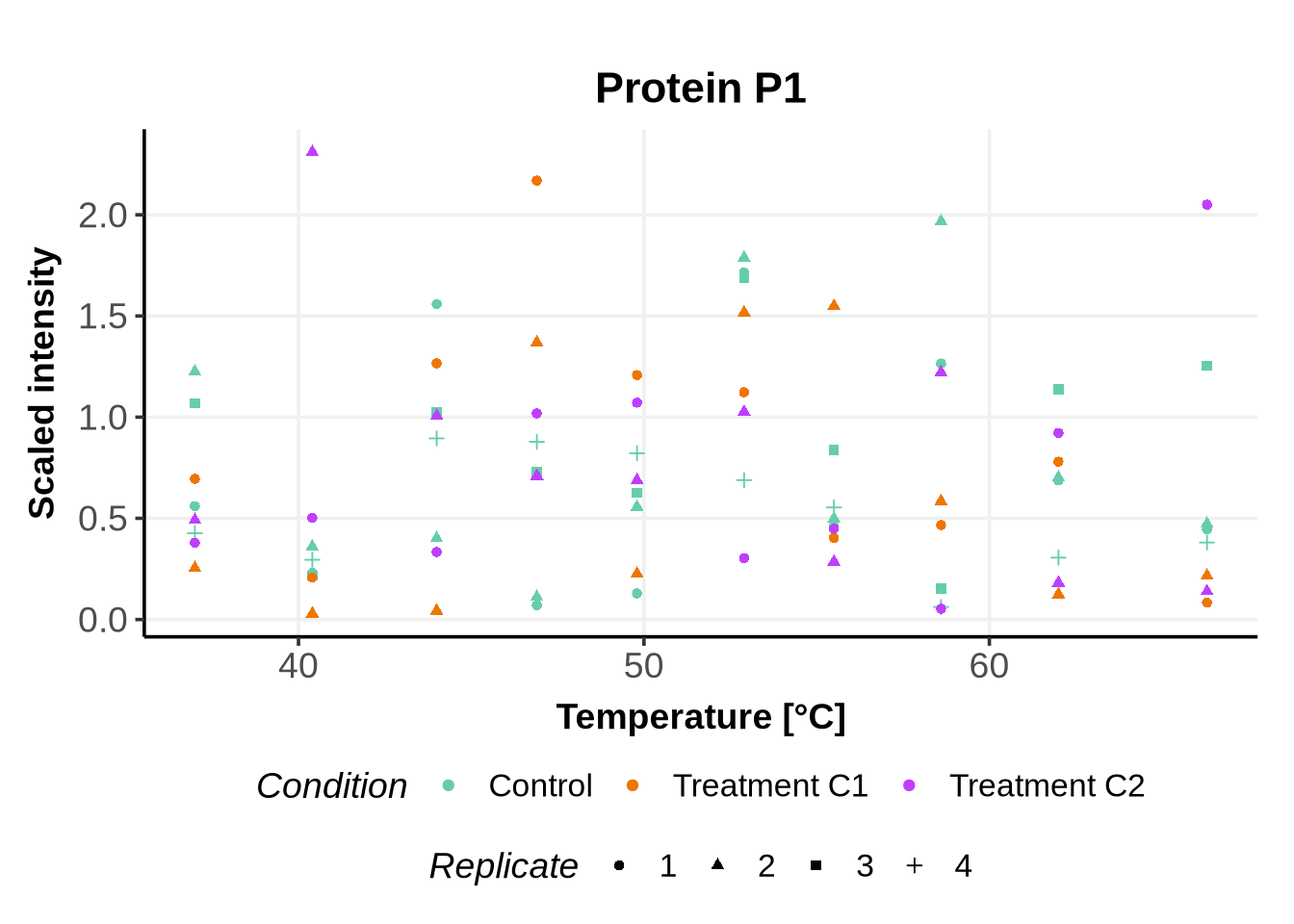
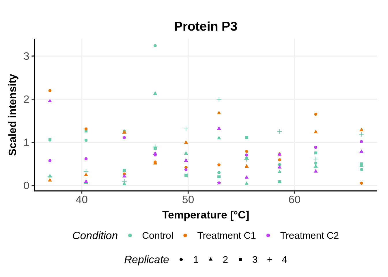
Before running GPMelt, we encourage users to check how the preprocessed data looks (at least a random sample of it). We propose below three visualisations along with the code to generate them.
5.1 All conditions and replicates together
Code
for(ID in c("P1", "P2", "P3")){

  print(
    ggplot(dummy_dataset %>%
             filter(Level_1==ID))+
      geom_point(aes(x=x, y = y, color = as.factor(Level_2), shape = as.factor(rep)))+
        scale_color_manual(name="Condition",
                     values = c("treatment_C1"="darkorange2",
                                "treatment_C2"="darkorchid1",
                                "control" = "aquamarine3"
                                ),
                     labels= c("treatment_C1" = "Treatment C1",
                               "treatment_C2"="Treatment C2",
                               "control"="Control"
                                ),
                     breaks =c("control","treatment_C1", "treatment_C2"))+
       xlab("Temperature [°C]")+
      ylab("Scaled intensity")+
     ggtitle(paste0("Protein ", ID))+
        theme_Publication()+
      guides(shape = guide_legend(title = "Replicate"))+
    theme(plot.title = element_text(hjust = 0.5),
          plot.subtitle = element_text(hjust = 0.5),
          legend.position = "bottom",
          legend.box="vertical",
          legend.margin=margin()
          )


  )
}

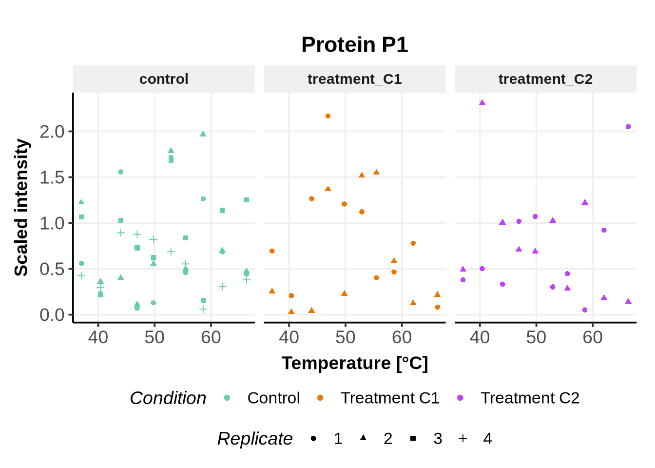
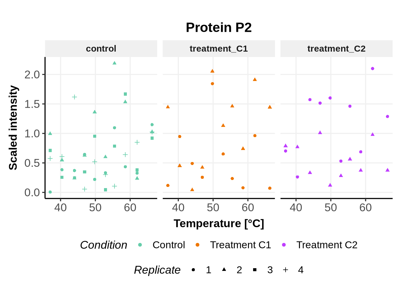
5.2 Each condition separately
Code
for(ID in c("P1", "P2", "P3")){

  print(
    ggplot(dummy_dataset %>%
             filter(Level_1==ID))+
      geom_point(aes(x=x, y = y, color = as.factor(Level_2), shape = as.factor(rep)))+
        scale_color_manual(name="Condition",
                     values = c("treatment_C1"="darkorange2",
                                "treatment_C2"="darkorchid1",
                                "control" = "aquamarine3"
                                ),
                     labels= c("treatment_C1" = "Treatment C1",
                               "treatment_C2"="Treatment C2",
                               "control"="Control"
                                ),
                     breaks =c("control","treatment_C1", "treatment_C2"))+
       xlab("Temperature [°C]")+
      ylab("Scaled intensity")+
     ggtitle(paste0("Protein ", ID))+
        theme_Publication()+
      guides(shape = guide_legend(title = "Replicate"))+
      facet_grid(.~Level_2)+
    theme(plot.title = element_text(hjust = 0.5),
          plot.subtitle = element_text(hjust = 0.5),
          legend.position = "bottom",
          legend.box="vertical",
          legend.margin=margin()
          )


  )
}

5.3 The three proteins together, each condition separately
Code
  print(
    ggplot(dummy_dataset)+
      geom_point(aes(x=x, y = y, color = as.factor(Level_2), shape = as.factor(rep)))+
        scale_color_manual(name="Condition",
                     values = c("treatment_C1"="darkorange2",
                                "treatment_C2"="darkorchid1",
                                "control" = "aquamarine3"
                                ),
                     labels= c("treatment_C1" = "Treatment C1",
                               "treatment_C2"="Treatment C2",
                               "control"="Control"
                                ),
                     breaks =c("control","treatment_C1", "treatment_C2"))+
       xlab("Temperature [°C]")+
      ylab("Scaled intensity")+
        theme_Publication()+
      guides(shape = guide_legend(title = "Replicate"))+
      facet_grid(Level_1~Level_2)+
    theme(plot.title = element_text(hjust = 0.5),
          plot.subtitle = element_text(hjust = 0.5),
          legend.position = "bottom",
          legend.box="vertical",
          legend.margin=margin()
          )


  )
6 Save the data
If the previous plots look fine, we can proceed by saving the data in the appropriate location.
For the purpose of this tutorial, we save them in the folder Nextflow/dummy_data/tutorial_dataset, using the filename dataForGPMelt.csv:
write.csv(dummy_dataset,
          file ="Nextflow/dummy_data/tutorial_dataset/dataForGPMelt.csv")
7 Session info
sessionInfo()R version 4.4.1 (2024-06-14)
Platform: x86_64-conda-linux-gnu
Running under: Debian GNU/Linux 12 (bookworm)
Matrix products: default
BLAS/LAPACK: /opt/conda/lib/libopenblasp-r0.3.27.so; LAPACK version 3.12.0
locale:
[1] LC_CTYPE=C.UTF-8 LC_NUMERIC=C LC_TIME=C.UTF-8
[4] LC_COLLATE=C.UTF-8 LC_MONETARY=C.UTF-8 LC_MESSAGES=C.UTF-8
[7] LC_PAPER=C.UTF-8 LC_NAME=C LC_ADDRESS=C
[10] LC_TELEPHONE=C LC_MEASUREMENT=C.UTF-8 LC_IDENTIFICATION=C
time zone: Etc/UTC
tzcode source: system (glibc)
attached base packages:
[1] stats graphics grDevices utils datasets methods base
other attached packages:
[1] ggplot2_3.5.1 dplyr_1.1.4
loaded via a namespace (and not attached):
[1] vctrs_0.6.5 cli_3.6.3 knitr_1.48 rlang_1.1.4
[5] xfun_0.48 purrr_1.0.2 generics_0.1.3 jsonlite_1.8.9
[9] labeling_0.4.3 glue_1.8.0 colorspace_2.1-1 htmltools_0.5.8.1
[13] scales_1.3.0 fansi_1.0.6 rmarkdown_2.28 grid_4.4.1
[17] munsell_0.5.1 evaluate_1.0.1 tibble_3.2.1 fastmap_1.2.0
[21] yaml_2.3.10 lifecycle_1.0.4 compiler_4.4.1 htmlwidgets_1.6.4
[25] pkgconfig_2.0.3 tidyr_1.3.1 farver_2.1.2 digest_0.6.37
[29] R6_2.5.1 tidyselect_1.2.1 utf8_1.2.4 pillar_1.9.0
[33] magrittr_2.0.3 withr_3.0.1 tools_4.4.1 gtable_0.3.5 References
Le Sueur, Cecile, Magnus Rattray, and Mikhail Savitski. 2024. “GPMelt: A Hierarchical Gaussian Process Framework to Explore the Dark Meltome of Thermal Proteome Profiling Experiments.” PLOS Computational Biology 20 (9): e1011632.