Matching variables names to the GPMelt nomenclature

1 Introduction

Although originally developed to model TPP-TR datasets, GPMelt is broadly applicable to any time-series datasets with replicates and conditions. For this reason, the naming conventions used in GPMelt have been designed to be general.

In this step, we will learn how to redefine the variables of a dataset to match the GPMelt nomenclature.

2 From experiments to hierarchy

The GPMelt framework is based on the idea of translating the experimental design parameters of an experiment (e.g. a biological protocol) into a hierarchy. By experimental design parameters, we refer to information such as replicates, conditions, batches, and more.

To translate these experimental design parameters into a hierarchy, the user needs to identify each level of the hierarchy, with Level_1 being the top of the hierarchy and Level_L the bottom level, where \(L\) is the number of levels in the hierarchy (e.g. \(L=3\) for a three-level hierarchical Gaussian process (HGP) model, \(L=4\) for a four-level HGP model).

We refer the reader to this page for a detailed explanation.

2.1 One possible translation

We illustrate hereafter how to translate the experimental design parameters of the ATP 2019 into levels of the hierarchy.

It is important to understand that these parameters carry a-priori knowledge on expected similarities between the modeled curves.

For example, an experimental design with replicates & conditions for each ID can be translated in a three-level HGP model, translating the following assumptions:

  • The bottom level of the hierarchy (Level_3) corresponds to the individual replicates. They are the leaves of the hierarchy: observations measured through a replicate (i.e at different temperatures for TPP-TR or different time points for a time-series dataset) are expected to be correlated. By correlated, we mean that each observation is expected to carry some information to help predicting the surrounding observations.
  • Observations from replicates coming from the same condition are expected to be similar, and this similarity can be captured by measuring the correlations between these replicates. Hence the second level of the hierarchy (Level_2) corresponds to the conditions.
  • Finally, observations from replicates coming from any conditions but one ID have the potential to share more similarities than observations from a different ID. For this reason, the top level of the hierarchy (Level_1) corresponds to the ID.

Note: This is one possible translation of the data into a hierarchy. If you have different hypotheses about your data, the levels of the hierarchy should be adjusted accordingly.

3 Renaming the variables

Below is a summary of the content of the dataset for each protein_id. By content, we mean the number of observations per replicate, denoted NumberOfTemperatures:

Data_forPython %>% 
  group_by(protein_id,gene_name, condition, replicate) %>% 
  summarise(NumberOfTemperatures = n_distinct(temperature)) %>%
  head(n = 10)
# A tibble: 10 × 5
# Groups:   protein_id, gene_name, condition [5]
   protein_id                 gene_name condition replicate NumberOfTemperatures
   <chr>                      <chr>     <chr>     <chr>                    <int>
 1 A0A087WZX2|O95139          NDUFB6    10mM_Mg_… 1                           10
 2 A0A087WZX2|O95139          NDUFB6    10mM_Mg_… 2                           10
 3 A0A087WZX2|O95139          NDUFB6    Vehicle   1                           10
 4 A0A087WZX2|O95139          NDUFB6    Vehicle   2                           10
 5 A0A096LP25|Q2M2I8-2|Q2M2I8 AAK1      10mM_Mg_… 1                           10
 6 A0A096LP25|Q2M2I8-2|Q2M2I8 AAK1      10mM_Mg_… 2                           10
 7 A0A096LP25|Q2M2I8-2|Q2M2I8 AAK1      Vehicle   1                           10
 8 A0A096LP25|Q2M2I8-2|Q2M2I8 AAK1      Vehicle   2                           10
 9 A2A2Q9|Q9Y312              AAR2      10mM_Mg_… 1                           10
10 A2A2Q9|Q9Y312              AAR2      10mM_Mg_… 2                           10

3.1 Level_3 of the hierarchy

In the present case, we aim to fit a melting curve to each replicate of each condition. This corresponds to the bottom level in the hierarchy.

There is not yet a variable in the data frame describing this level. Let’s create it by combining the condition information and the replicate index:

Data_forPython <- Data_forPython %>%
  tidyr::unite(col="Level_3", condition,replicate, sep=".", remove=FALSE)

head(Data_forPython)
# A tibble: 6 × 7
  protein_id      gene_name Level_3       condition replicate     FC temperature
  <chr>           <chr>     <chr>         <chr>     <chr>      <dbl>       <dbl>
1 Q6PD74|Q6PD74-2 AAGAB     10mM_Mg_ATP.1 10mM_Mg_… 1         0.998         37  
2 Q6PD74|Q6PD74-2 AAGAB     10mM_Mg_ATP.1 10mM_Mg_… 1         0.857         44  
3 Q6PD74|Q6PD74-2 AAGAB     10mM_Mg_ATP.1 10mM_Mg_… 1         0.996         40.4
4 Q6PD74|Q6PD74-2 AAGAB     10mM_Mg_ATP.1 10mM_Mg_… 1         0.349         49.8
5 Q6PD74|Q6PD74-2 AAGAB     10mM_Mg_ATP.1 10mM_Mg_… 1         0.744         46.9
6 Q6PD74|Q6PD74-2 AAGAB     10mM_Mg_ATP.1 10mM_Mg_… 1         0.0485        55.5

The newly created Level_3 variable takes the following values:

Code
unique(Data_forPython$Level_3)
[1] "10mM_Mg_ATP.1" "Vehicle.1"     "10mM_Mg_ATP.2" "Vehicle.2"    

3.2 Level_2 of the hierarchy

Leveraging the principle of hierarchical models, we aim to improve the individual replicates fits by sharing information between replicates within a condition.

To translate this assumption in terms of hierarchy, we add a second level, which captures which replicate belongs to which condition.

This second level is directly given by the variable condition. Let’s rename this variable Level_2.

Data_forPython <- Data_forPython %>%
  dplyr::rename("Level_2" = "condition")

head(Data_forPython)
# A tibble: 6 × 7
  protein_id      gene_name Level_3       Level_2   replicate     FC temperature
  <chr>           <chr>     <chr>         <chr>     <chr>      <dbl>       <dbl>
1 Q6PD74|Q6PD74-2 AAGAB     10mM_Mg_ATP.1 10mM_Mg_… 1         0.998         37  
2 Q6PD74|Q6PD74-2 AAGAB     10mM_Mg_ATP.1 10mM_Mg_… 1         0.857         44  
3 Q6PD74|Q6PD74-2 AAGAB     10mM_Mg_ATP.1 10mM_Mg_… 1         0.996         40.4
4 Q6PD74|Q6PD74-2 AAGAB     10mM_Mg_ATP.1 10mM_Mg_… 1         0.349         49.8
5 Q6PD74|Q6PD74-2 AAGAB     10mM_Mg_ATP.1 10mM_Mg_… 1         0.744         46.9
6 Q6PD74|Q6PD74-2 AAGAB     10mM_Mg_ATP.1 10mM_Mg_… 1         0.0485        55.5

3.3 Level_1 of the hierarchy

Finally, we hypothesis that observations from replicates across different conditions but within the same ID may share more similarities than those from different IDs.

Typically, if the treatment condition(s) have no effect, we would expect the melting curves across all conditions to be similar and therefore strongly correlated.

To translate this assumption in our model, we define the IDs as the top level of the hierarchy. This will allow information sharing between replicates across different conditions within each ID.

Let’s rename the variable gene_name by Level_1:

Data_forPython <- Data_forPython %>%
  dplyr::rename("Level_1" = "gene_name") %>%
  mutate(Level_1 = gsub("/|\\._" , "-", Level_1, fixed=TRUE)) #names with  slash can be annoying

head(Data_forPython)
# A tibble: 6 × 7
  protein_id      Level_1 Level_3       Level_2     replicate     FC temperature
  <chr>           <chr>   <chr>         <chr>       <chr>      <dbl>       <dbl>
1 Q6PD74|Q6PD74-2 AAGAB   10mM_Mg_ATP.1 10mM_Mg_ATP 1         0.998         37  
2 Q6PD74|Q6PD74-2 AAGAB   10mM_Mg_ATP.1 10mM_Mg_ATP 1         0.857         44  
3 Q6PD74|Q6PD74-2 AAGAB   10mM_Mg_ATP.1 10mM_Mg_ATP 1         0.996         40.4
4 Q6PD74|Q6PD74-2 AAGAB   10mM_Mg_ATP.1 10mM_Mg_ATP 1         0.349         49.8
5 Q6PD74|Q6PD74-2 AAGAB   10mM_Mg_ATP.1 10mM_Mg_ATP 1         0.744         46.9
6 Q6PD74|Q6PD74-2 AAGAB   10mM_Mg_ATP.1 10mM_Mg_ATP 1         0.0485        55.5

3.4 Variable condition

An additional variable condition can be added to the dataset. For this variable, only the control condition will have the exact same value for both condition and Level_2.

Let’s add this variable:

Data_forPython <- Data_forPython %>%
  mutate(condition = ifelse(Level_2 == "Vehicle", "Vehicle", "Treatment" ))

head(Data_forPython)
# A tibble: 6 × 8
  protein_id      Level_1 Level_3 Level_2 replicate     FC temperature condition
  <chr>           <chr>   <chr>   <chr>   <chr>      <dbl>       <dbl> <chr>    
1 Q6PD74|Q6PD74-2 AAGAB   10mM_M… 10mM_M… 1         0.998         37   Treatment
2 Q6PD74|Q6PD74-2 AAGAB   10mM_M… 10mM_M… 1         0.857         44   Treatment
3 Q6PD74|Q6PD74-2 AAGAB   10mM_M… 10mM_M… 1         0.996         40.4 Treatment
4 Q6PD74|Q6PD74-2 AAGAB   10mM_M… 10mM_M… 1         0.349         49.8 Treatment
5 Q6PD74|Q6PD74-2 AAGAB   10mM_M… 10mM_M… 1         0.744         46.9 Treatment
6 Q6PD74|Q6PD74-2 AAGAB   10mM_M… 10mM_M… 1         0.0485        55.5 Treatment

This condition variable is especially useful when more than one treatment condition is measured. In this case, the condition variable differentiates between control and treatment, while the Level_2 variable specifies the different treatment conditions.

Code
Data_forPython %>% 
  dplyr::select(Level_1,Level_2,condition) %>% 
  distinct() 
# A tibble: 32 × 3
   Level_1 Level_2     condition
   <chr>   <chr>       <chr>    
 1 AAGAB   10mM_Mg_ATP Treatment
 2 AAGAB   Vehicle     Vehicle  
 3 AAK1    10mM_Mg_ATP Treatment
 4 AAK1    Vehicle     Vehicle  
 5 AAMDC   10mM_Mg_ATP Treatment
 6 AAMDC   Vehicle     Vehicle  
 7 AAMP    10mM_Mg_ATP Treatment
 8 AAMP    Vehicle     Vehicle  
 9 AAR2    10mM_Mg_ATP Treatment
10 AAR2    Vehicle     Vehicle  
# ℹ 22 more rows

3.5 Replicate, temperature and scaled intensity

To match the variables names in GPMelt implementation, we rename the replicate, temperature and FC columns:

Data_forPython <- Data_forPython %>%
  dplyr::rename("rep"="replicate",
                "x"="temperature",
                "y"="FC")

head(Data_forPython)
# A tibble: 6 × 8
  protein_id      Level_1 Level_3       Level_2     rep        y     x condition
  <chr>           <chr>   <chr>         <chr>       <chr>  <dbl> <dbl> <chr>    
1 Q6PD74|Q6PD74-2 AAGAB   10mM_Mg_ATP.1 10mM_Mg_ATP 1     0.998   37   Treatment
2 Q6PD74|Q6PD74-2 AAGAB   10mM_Mg_ATP.1 10mM_Mg_ATP 1     0.857   44   Treatment
3 Q6PD74|Q6PD74-2 AAGAB   10mM_Mg_ATP.1 10mM_Mg_ATP 1     0.996   40.4 Treatment
4 Q6PD74|Q6PD74-2 AAGAB   10mM_Mg_ATP.1 10mM_Mg_ATP 1     0.349   49.8 Treatment
5 Q6PD74|Q6PD74-2 AAGAB   10mM_Mg_ATP.1 10mM_Mg_ATP 1     0.744   46.9 Treatment
6 Q6PD74|Q6PD74-2 AAGAB   10mM_Mg_ATP.1 10mM_Mg_ATP 1     0.0485  55.5 Treatment

Note that we use the variable name y without specifying the scaling method used to scale the intensities: this makes GPMelt applicable with any scaling method (see scaling methods explained here)

3.6 Variables ordering

For ease of readability, we can reorder the variables:

Data_forPython <- Data_forPython %>%
  dplyr::relocate(protein_id, Level_1, condition, Level_2,  Level_3, rep, x, y)
  
head(Data_forPython)
# A tibble: 6 × 8
  protein_id      Level_1 condition Level_2     Level_3       rep       x      y
  <chr>           <chr>   <chr>     <chr>       <chr>         <chr> <dbl>  <dbl>
1 Q6PD74|Q6PD74-2 AAGAB   Treatment 10mM_Mg_ATP 10mM_Mg_ATP.1 1      37   0.998 
2 Q6PD74|Q6PD74-2 AAGAB   Treatment 10mM_Mg_ATP 10mM_Mg_ATP.1 1      44   0.857 
3 Q6PD74|Q6PD74-2 AAGAB   Treatment 10mM_Mg_ATP 10mM_Mg_ATP.1 1      40.4 0.996 
4 Q6PD74|Q6PD74-2 AAGAB   Treatment 10mM_Mg_ATP 10mM_Mg_ATP.1 1      49.8 0.349 
5 Q6PD74|Q6PD74-2 AAGAB   Treatment 10mM_Mg_ATP 10mM_Mg_ATP.1 1      46.9 0.744 
6 Q6PD74|Q6PD74-2 AAGAB   Treatment 10mM_Mg_ATP 10mM_Mg_ATP.1 1      55.5 0.0485

3.7 Variables sorting

To ensure that the Python code correctly handles the data, the input data should be properly sorted. The dataset will be sorted using the following variables in this specific order (this step is handled directly in the Nextflow pipeline, no need to do it manually):

  1. Level_1
  2. condition
  3. Level_2
  4. Level_3
  5. rep (replicate)
  6. x (temperature)

4 Check the data

Before running GPMelt, we strongly encourage you to check how the preprocessed data look like.

Here is an example R code to do so. See here, section 5 for more examples of R codes.

for(ID in c("AAGAB", "CDK13", "DPM1", "AAK1", "AAMDC", "AAMP", "AAR2", "NDUFB6" ,"MYO1G","BANF1", "DDX50", "FBL", "NOP56", "EIF3H", "IMPDH1", "NUCKS1")){
  
  print(
    ggplot(Data_forPython %>%
             filter(Level_1==ID))+
    geom_point(aes(x=x, y= y, color = as.factor(condition), shape = as.factor(rep)))+
    scale_color_manual(name="Condition",
                       values = c("Treatment"="darkorange2",
                                "Vehicle" = "aquamarine3",
                                "joint"="black"
                                ),
                       labels= c("Treatment" = "Treatment (10mM Mg-ATP)",
                               "Vehicle"="Vehicle",
                               "joint"="Joint"
                                ),
                       breaks =c("Treatment", "Vehicle", "joint"))+
    xlab("Temperature [°C]")+
    ylab("Fold Change")+
    ggtitle(paste0("Protein ", ID))+
    theme_Publication()+
    guides(shape = guide_legend(title = "Replicate"))+
    theme(plot.title = element_text(hjust = 0.5),
          plot.subtitle = element_text(hjust = 0.5),
          legend.position = "bottom",
          legend.box="vertical", 
          legend.margin=margin()
          )

    
  )
}

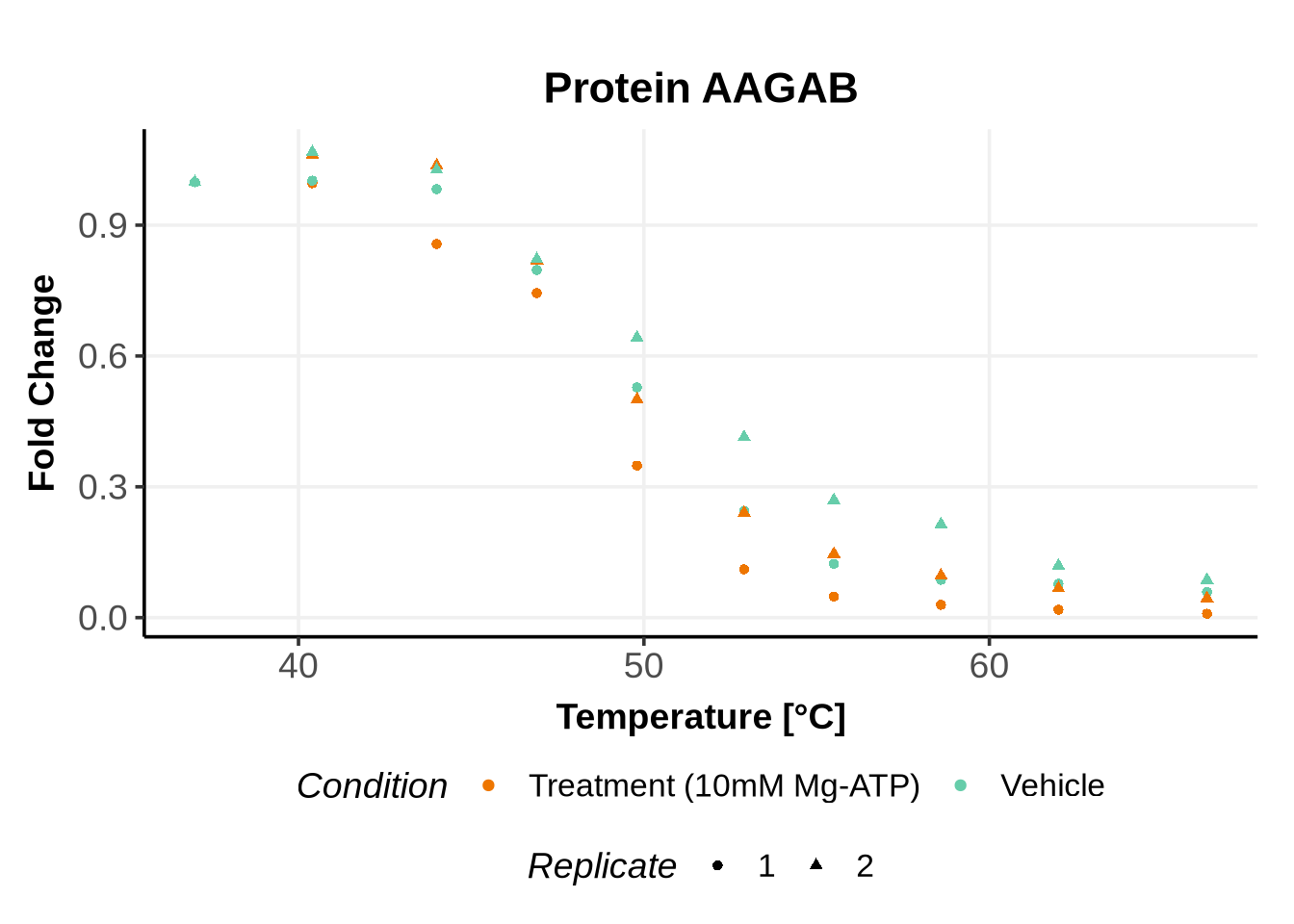
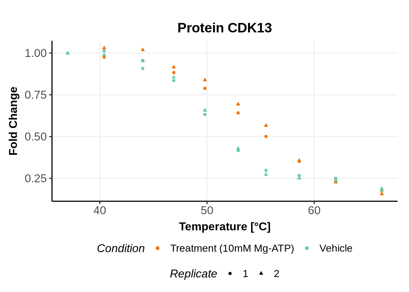
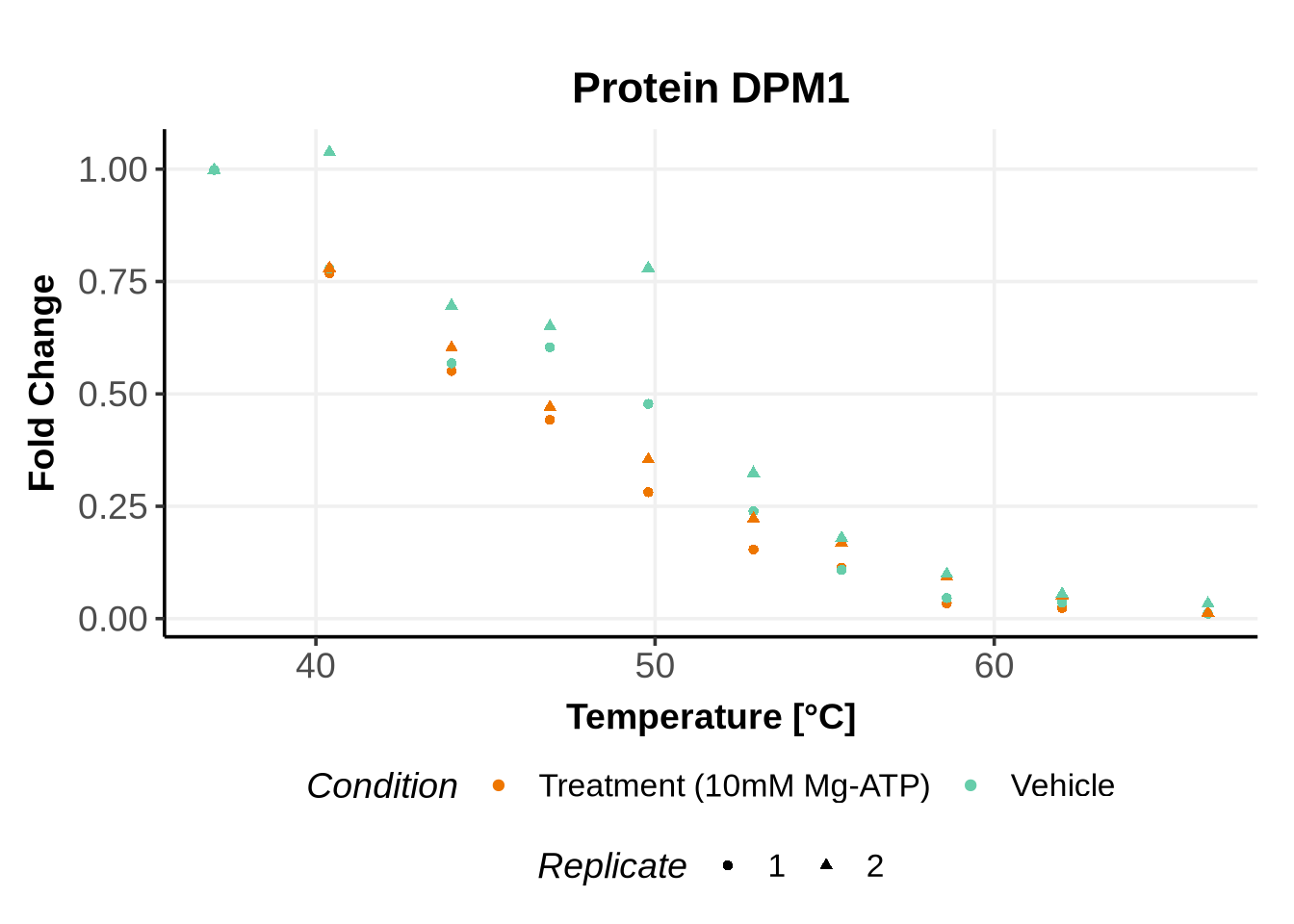
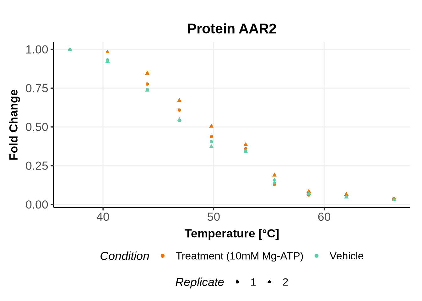
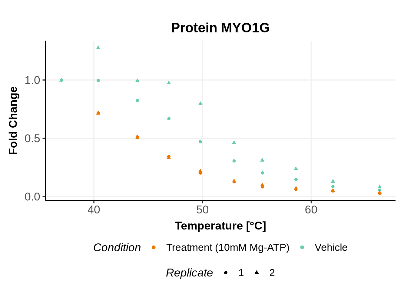
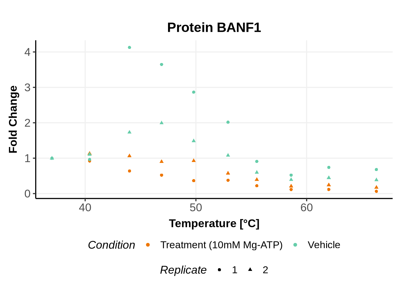
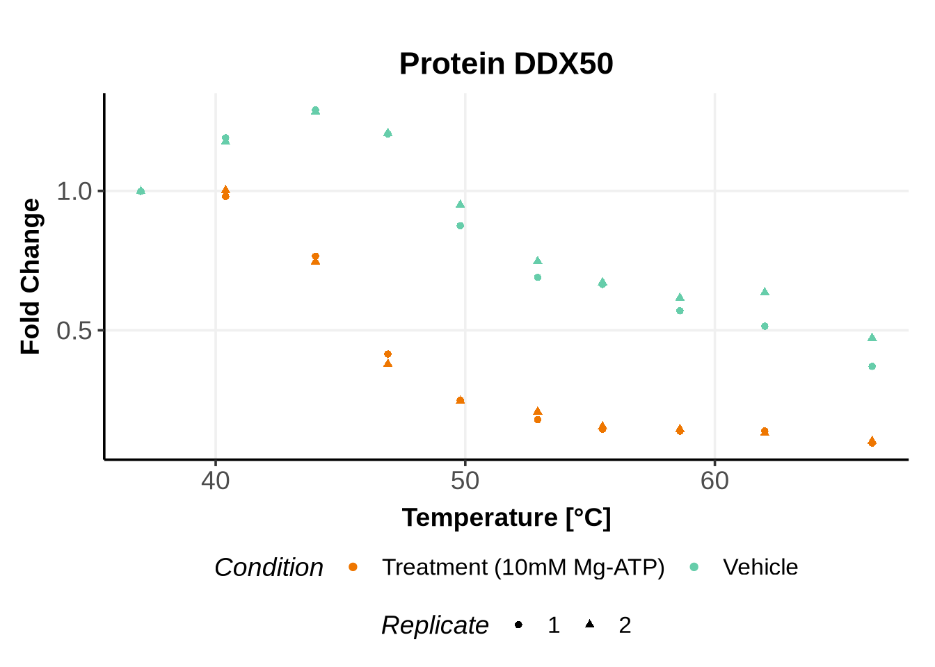
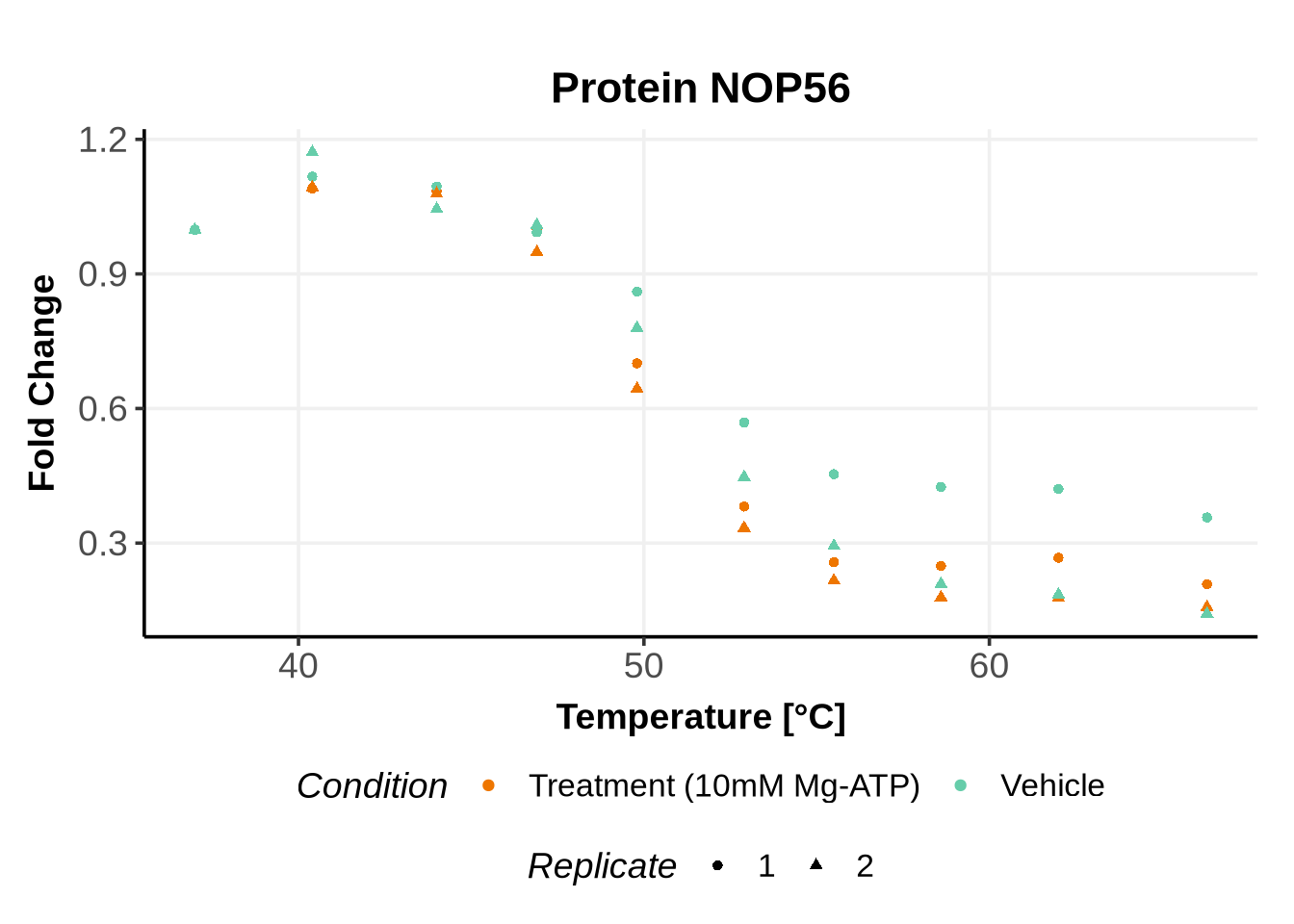
In the previous code, we selected a set of proteins which can be used to further test different model specifications.

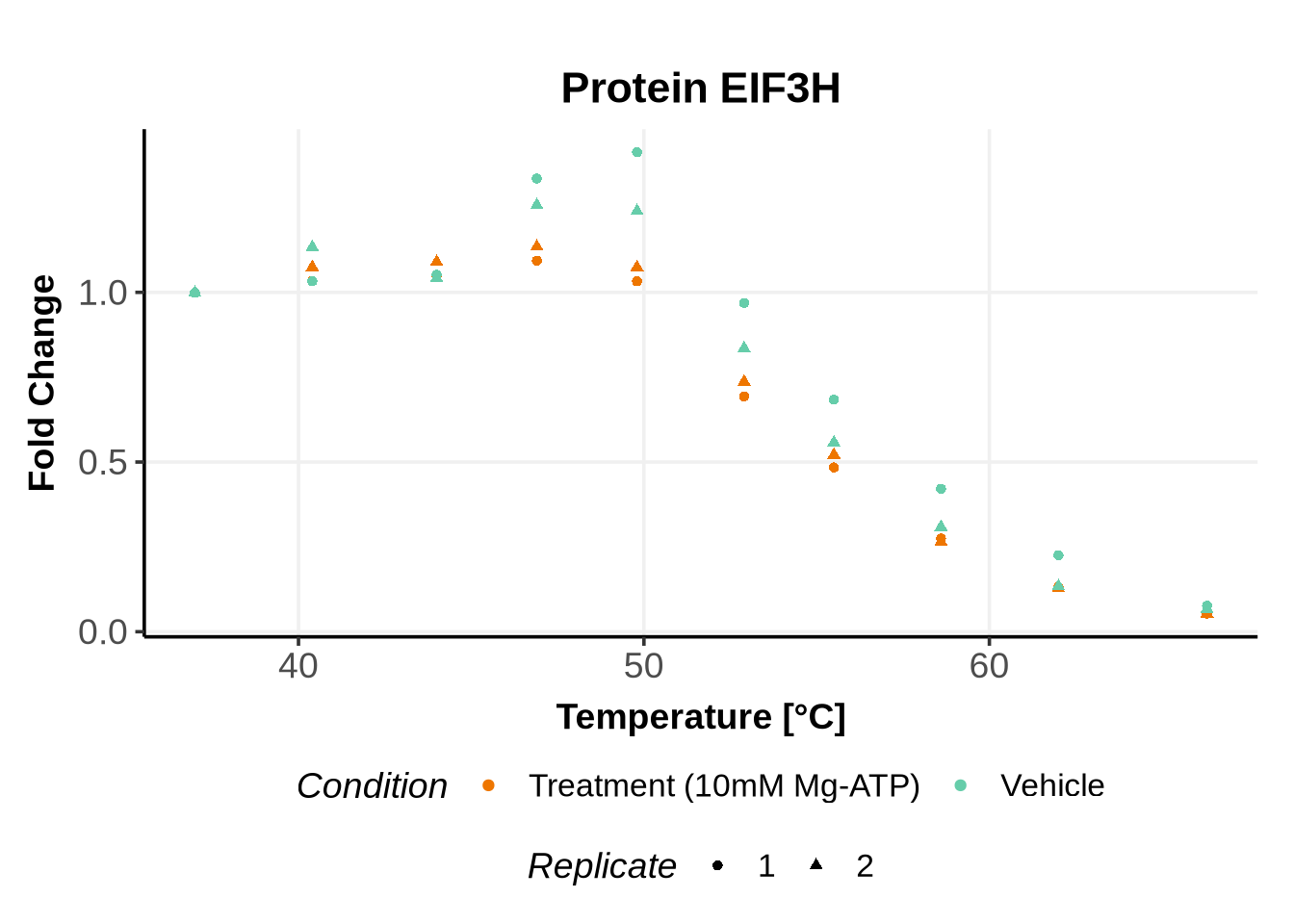
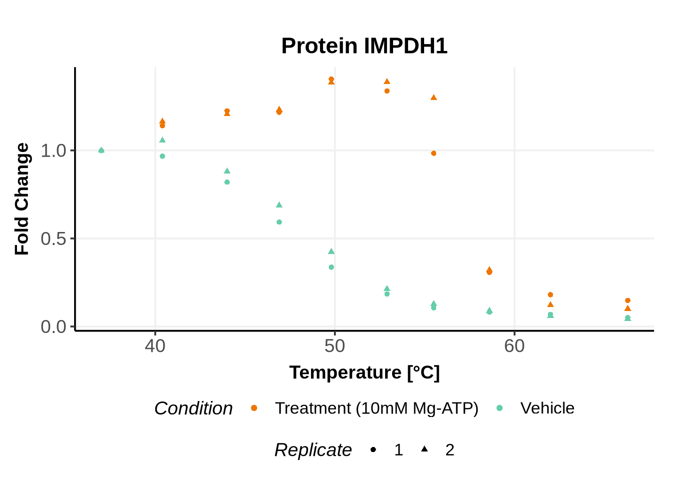
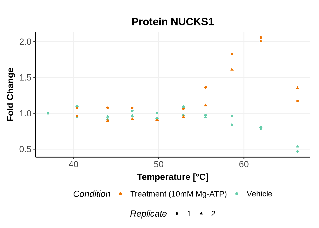
We selected IDs with different melting curve patterns (sigmoidal and non-sigmoidal), and different levels of noise (e.g. BANF1 present an outlier replicate, the vehicle condition of MYO1G and NDUFB6 are also noisy, while other IDs like IMPDH1 or AAR2 have well-reproducible replicates). Comparing the quality of the fits for these IDs will help us deciding how to update the model specification if needed (see here).

If you have no idea of the IDs you want to use to test the model specification, you can randomly pick names of IDs in the dataset:

set.seed(837456) # for reproducibility
RandomSample <- sample(unique(Data_forPython$Level_1), size=10) # randomly select 10 names from the Level_1

5 Save the data

We then save the data in the folder Nextflow/dummy_data/ATP2019, using the name dataForGPMelt.csv:

write.csv(Data_forPython,
          file ="Nextflow/dummy_data/ATP2019/dataForGPMelt.csv")