Adapting model complexity

1 Introduction

Not all GPMelt models are expected to be complex. Protein-level TPP-TR datasets with two or three conditions and two to four replicates, as described in GPMelt (Le Sueur, Rattray, and Savitski 2024) are relatively simple, and likely present a unique (or prevalent) log marginal likelihood optimum.

However, when modelling a scenario with multiple conditions and each condition presenting multiple replicates, using potentially deeper hierarchies with four or more levels, the model will be complex. In the previous page, we discuss the presence of multiple local optima for complex models.

One strength of GPMelt lies in its capacity to model simple to very complex experimental protocols. To improve the convergence of complex models, we discuss hereafter how we can further simplify (or complexify) a model specification in case the model presents too many local optima, with potentially too many parameters to estimate.

In the following, we consider a hierarchical model with \(L\) levels, level \(1\) being the top of the hierarchy (e.g. the protein level) and level \(L\) representing the leaves of the hierarchy (e.g. the replicates level).

2 One or multiple lengthscale(s)?

In the current GPMelt implementation, we can choose to use one or two lengthscales in the model.

The first lengthscale, denoted \(\lambda_1\), will be used to model levels \(1\) to \(L-1\). If a second lengthscale, denoted \(\lambda_2\), is used, then it will model level \(L\), i.e. the leaves of the hierarchy.

2.1 Why would we need to use two lengthscales?

While \(\lambda_1\) captures slow variations, corresponding to the general trends in the data, \(\lambda_2\) helps capture fast variations in the melting curves of the leaves of the hierarchy.

If a large replicates-to-replicates variability is observed, and/or a lot of correlated noise is observed on the replicate level¹, it may be useful to capture these fast variations with \(\lambda_2\), such that \(\lambda_1\) can more robustly capture the general (slower) trend.

Therefore, we recommend first considering the results of the simplest model with \(\lambda_{1} \equiv \lambda_{2}\) and only relaxing the constraint on \(\lambda_{2}\) if fast variations in the replicates’ melting curves are too poorly captured.

3 One or multiple output-scale(s)?

Similarly, in the current GPMelt implementation, the output-scales of the lower levels can either be shared across all tasks (e.g. one task = one replicate) or be unique to each task.

To make this decision, it is essential to understand that the output-scale measures how much a particular task deviates from the general trend.

Consider a three-level HGP model. The replicates’ output-scales indicate how much each replicate deviates from the condition-wise melting curve, which represents the trend for all replicates within that condition.

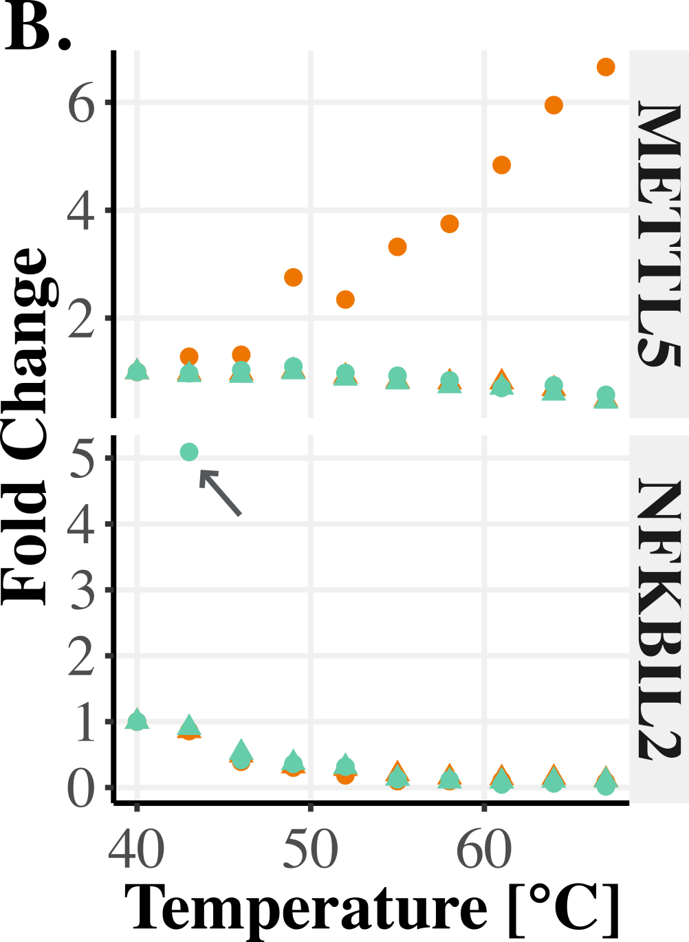
Therefore, releasing the constraint on the output-scale for the last level of the hierarchy allows better capture of noise in the amplitudes of the curves. For instance, the output-scale can capture whether some replicates contain outlier observations or if entire replicates behave as outliers (see Figure 1).

By capturing these deviations through the replicate-specific output-scale, the general fit becomes more robust, as the parameters describing the general behavior of the curves do not need to account for outlier data

Figure 1: Outliers observations can be modeled with large output-scales. This figure illustrates two real examples from the Staurosporine dataset Savitski et al. (2014). METTL5 is an example of a correlated noise with large amplitude, where only one replicate out of four is strongly deviating from the general trend. Below, NFKBIL2 illustrates a ponctual outlier observation with large amplitude. Both cases can be captured by allowing output-scales to vary across replicates. This way, only the replicates containing the outliers will be associated with a very large estimated value of output-scale, and the general trend will be captured more robustly. Panel B reproduced from Figure 6 of (Le Sueur, Rattray, and Savitski 2024).

References

Le Sueur, Cecile, Magnus Rattray, and Mikhail Savitski. 2024. “GPMelt: A Hierarchical Gaussian Process Framework to Explore the Dark Meltome of Thermal Proteome Profiling Experiments.” PLOS Computational Biology 20 (9): e1011632.

Savitski, Mikhail M, Friedrich BM Reinhard, Holger Franken, Thilo Werner, Maria Fälth Savitski, Dirk Eberhard, Daniel Martinez Molina, et al. 2014. “Tracking Cancer Drugs in Living Cells by Thermal Profiling of the Proteome.” Science 346 (6205): 1255784.

Footnotes

1. Uncorrelated noise means that the observations seem to randomly oscillate around the true trend. Correlated noise is observed when observations will coherently deviate from the true trend, for example a similar increase of intensity is seen for three consecutive temperatures, or a bump in intensity is observed, with the intensities first increasing and then descresing before starting again to randomly oscillate around the true trend.