Gaussian process hyper-parameters

1 Introduction

In Video 1, we introduced the concept of GP hyper-parameters.

For the purpose of this tutorial, we do not need to introduce the difference between parameters and hyper-parameters, and in the following, we consider these two notions as interchangeable.

GP’s hyper-parameters fully describe the GP behaviour. In the case of the GPMelt model, we only need to introduce \(4\) hyper-parameters:

• the mean \(\mu\),
• the lengthscale \(\lambda\) of the RBF¹ kernel,
• the output-scale \(\sigma^2\) of the RBF kernel,
• the noise variance \(\beta^2\).

2 Restating the GP regression

We state hereafter a simplified form of the GP regression used in the GPMelt model and illustrated in Video 1.

For \(i \in [1, N]\):

\[\begin{align} y_i &= f(t_i) + \epsilon_i \\ f(\cdot) &\sim GP( \mu(\cdot), k(\cdot, \cdot)) \\ \epsilon_i &\sim \mathcal{N}(0, \beta^2 I) \end{align}\]

3 R code for the upcoming plots

While the lengthscale \(\lambda\) and output-scale \(\sigma^2\) of the RBF kernels are likely the most important parameters in GP regression, we aim to give readers an intuition behind all GP parameters in Section 4 to Section 7.

For this, we use the R functions defined in Section 3.1 to Section 3.3 (unfold the code if desired), loading the following libraries:

library(ggplot2)
library(latex2exp)
source("../../utils.R")

3.1 RBF kernel

This function takes as input the following parameters:

• the vector of points \((x_{1}, x_{2})\)
• the lengthscale \(\lambda\) of the RBF kernel,
• the output-scale \(\sigma^2\) of the RBF kernel,

# code written with ChatGPT v4o
# RBF kernel function
rbf_kernel <- function(x1, x2, lambda, sigma_sq) {
  dist_sq <- outer(x1, x2, FUN = function(a, b) (a - b)^2)
  return(sigma_sq * exp(-dist_sq / (2 * lambda^2)))
}

3.2 Posterior distribution for a set of parameter

This function takes as input the following parameters:

• the training data \((X_{obs}, y_{obs})\),
• the lengthscale \(\lambda\) of the RBF kernel,
• the output-scale \(\sigma^2\) of the RBF kernel,
• the noise variance \(\beta^2\),
• the mean function \(\mu\),
• the number n_PredictionsPoints of test points, defined as evenly spaced between \(min(X_{obs})\) and \(max(X_{obs})\).

##########################
# gp_posterior_distri : computes the posterior distribution for the given hyper-parameters
# code written with ChatGPT v4o
##########################
gp_posterior_distri <- function(X_obs, y_obs, lambda, sigma_sq, beta_sq, prior_mean_func = function(x) 0, n_PredictionsPoints = 50) {
  
  # Covariance matrices
  K <- rbf_kernel(X_obs, X_obs, lambda, sigma_sq)  # Covariance between observed points
  K <- K + beta_sq * diag(length(X_obs))  # Add noise (likelihood variance)
  
  # Inverse of the covariance matrix
  K_inv <- solve(K)
  
  # Prediction points (new points for prediction)
  X_test <- seq(min(X_obs), max(X_obs), length.out = n_PredictionsPoints)
  
  # Covariance between test and observed points
  K_star <- rbf_kernel(X_test, X_obs, lambda, sigma_sq)
  
  # Covariance between test points
  K_star_star <- rbf_kernel(X_test, X_test, lambda, sigma_sq)
  
  # Prior mean for observed points and test points
  prior_mean_obs <- prior_mean_func(X_obs)
  prior_mean_test <- prior_mean_func(X_test)
  
  # Adjust y_obs by subtracting the prior mean
  y_adjusted <- y_obs - prior_mean_obs
  
  # Mean prediction: incorporates the prior mean at test points
  mu_star <- prior_mean_test + K_star %*% K_inv %*% y_adjusted
  
  # Variance prediction
  sigma_star_sq <- K_star_star - K_star %*% K_inv %*% t(K_star)
  sigma_star <- sqrt(diag(sigma_star_sq))  # Extract the diagonal as the standard deviation
  
  # 95% confidence intervals
  lower_bound <- mu_star - 1.96 * sigma_star
  upper_bound <- mu_star + 1.96 * sigma_star
  
  # Return a list with predictions, confidence intervals, and test points
  return(list(mean = mu_star, lower = lower_bound, upper = upper_bound, variance = sigma_star_sq, X_test = X_test))
}

3.3 Posterior distribution on a grid of parameters

This function call the previously defined function gp_posterior_distri on a grid of hyper-parameters:

• the training data \((X_{obs}, y_{obs})\),
• a vector of lengthscales \(\lambda\) for the RBF kernel,
• a vector of output-scales \(\sigma^2\) for the RBF kernel,
• a vector of noise variance \(\beta^2\) for the likelihood,
• a list of mean functions \(\mu\),
• the number n_PredictionsPoints of test points, defined as evenly spaced between \(min(X_{obs})\) and \(max(X_{obs})\).

##########################
# gp_grid_posterior_distri: computes the posterior distribution for any combination of hyper-parameters
# code written with ChatGPT v4o
##########################

# Function to run GP predictions for all combinations of lambda, sigma_sq, beta_sq
gp_grid_posterior_distri <- function(X_obs,
                                     y_obs, 
                                     lambda_vec, 
                                     sigma_sq_vec, 
                                     beta_sq_vec, 
                                     mean_func_list= list(function(x) 0),
                                     n_PredictionsPoints = 50) {
  
  # Generate a grid of all combinations of lambda, sigma_sq, and beta_sq
  param_grid <- expand.grid(lambda = lambda_vec, sigma_sq = sigma_sq_vec, beta_sq = beta_sq_vec, mean_func_idx = seq_along(mean_func_list))
  
  # Initialize an empty list to store the results
  results_list <- list()
  
  # Define a grid of test points to predict over
  X_test <- seq(min(X_obs), max(X_obs), length.out = n_PredictionsPoints)
  
  # Loop over all combinations of parameters
  for (i in 1:nrow(param_grid)) {
    
    # Extract the current parameter combination
    lambda <- param_grid$lambda[i]
    sigma_sq <- param_grid$sigma_sq[i]
    beta_sq <- param_grid$beta_sq[i]
    
    # Extract the corresponding mean function from the list
    prior_mean_func <- mean_func_list[[param_grid$mean_func_idx[i]]]
    

    # Perform GP prediction for the current combination
    gp_result <- gp_posterior_distri( X_obs, y_obs, lambda, sigma_sq, beta_sq,prior_mean_func, n_PredictionsPoints)
    
    # Store the results in a data frame, adding lambda, sigma_sq, and beta_sq as columns
    temp_df <- data.frame(
      x = X_test, 
      mean = gp_result$mean,
      lower = gp_result$lower,
      upper = gp_result$upper,
      variance = diag(gp_result$variance),
      lambda = lambda,
      sigma_sq = sigma_sq,
      beta_sq = beta_sq, 
      prior_mean_func = param_grid$mean_func_idx[i]
    )
    
    # Append the result to the list
    results_list[[i]] <- temp_df
  }
  
  # Combine all results into a single data frame
  result_df <- do.call(rbind, results_list)
  
  return(result_df)
}

3.4 Training data

We now consider the following training data representing some non-sigmoidal melting curves:

# Generate the specified x values
x <- seq(37.0,66.3, length.out = 50) 
x_obs <- c(37.0, 40.4, 44.0, 46.9, 49.8, 52.9, 55.5, 58.6, 62.0, 66.3)

# Transform the sine function to oscillate between 0 and 1.5 and add noise

y_func <- function(x){
  return((1.5 / 2) * (sin(1.8 * pi * (x - 37) / (66.3 - 37) + (1 *pi / 8) ) + 1) )
}

set.seed(123)  # For reproducibility

y <- y_func(x) 
y_obs <- y_func(x_obs) + rnorm(length(x_obs), sd = 0.15)

# Create a data frame to hold the x and y values
data <- data.frame(x = x, y = y)
data_obs <- data.frame(x_obs = x_obs, y_obs=y_obs)

# Plot the data to visualize the function
ggplot(data)+
  geom_line(data=data, aes(x=x, y=y, linetype ="dotted"), na.rm = TRUE)+
  geom_point(data= data_obs, aes(x=x_obs, y= y_obs, shape = "16" ), size=2, na.rm =TRUE)+
  scale_linetype_manual(name = "True function", values = c("dotted"="dotted") )+
  scale_shape_manual(name = "Observations", values = c("16"=16))+
  theme_Publication()+
  xlab("Temperature [°C]") +
  ylab("Scaled intensity") +
  theme(legend.text = element_blank())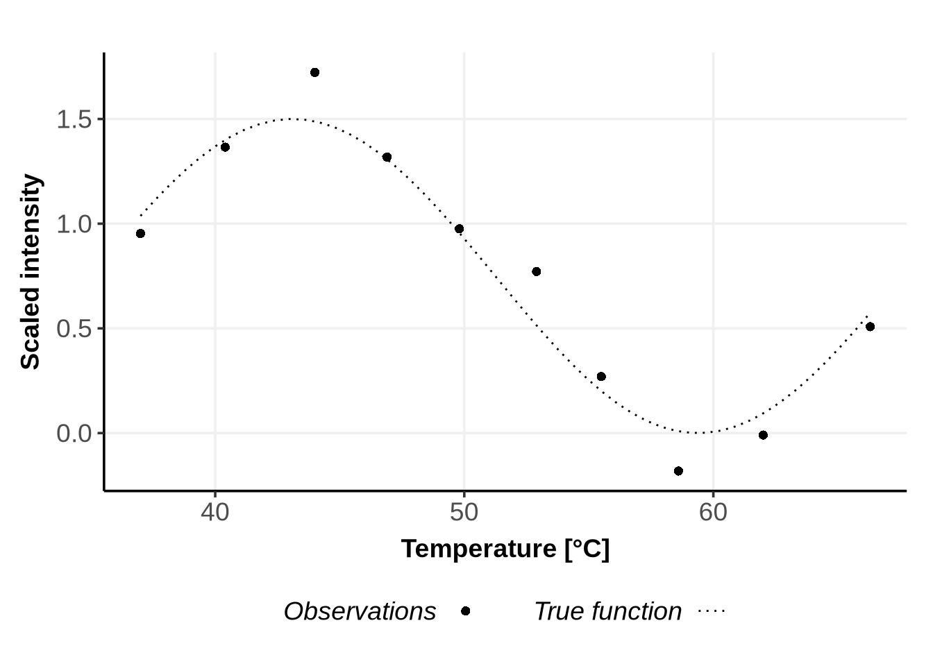

4 The lengthscale parameter

The lengthscale \(\lambda\) describes how fast the correlation decreases with the distance between two points. Short lengthscales describe rapidly varying functions, while longer lengthscales describe slowly varying functions.

lambda_vec <- c(1, 10, 20, 100)     # Lengthscale
sigma_sq_vec <- 1  # Output-scale 
beta_sq_vec <- 0.15^2  # Likelihood variance (same as noise level in y_obs)

gp_results_df <- gp_grid_posterior_distri(
  data_obs$x_obs, 
  data_obs$y_obs,
  lambda_vec, 
  sigma_sq_vec,
  beta_sq_vec,
  mean_func_list = list(function(x) 0),
  n_PredictionsPoints=50)

ggplot() +
  geom_line(data = gp_results_df, aes(x = x, y = mean), color = "black") +
  geom_ribbon(data = gp_results_df,
              aes(x = x, ymin = lower, ymax = upper), fill = "grey", alpha = 0.4) +
  geom_point(data = data_obs, aes(x = x_obs, y = y_obs), na.rm = TRUE, color = "black") +
  facet_grid(.~lambda, labeller = label_bquote(cols = lambda == .(lambda)))+
  xlab("Temperature [°C]") +
  ylab("Scaled intensity") +
  ggtitle("Posterior distribution for varying lengthscale parameters",
          subtitle = TeX(paste0("$\\mu \\equiv 0$, $\\sigma^2 = $", sigma_sq_vec, " and $\\beta^2 = $", beta_sq_vec )))+
  theme_Publication()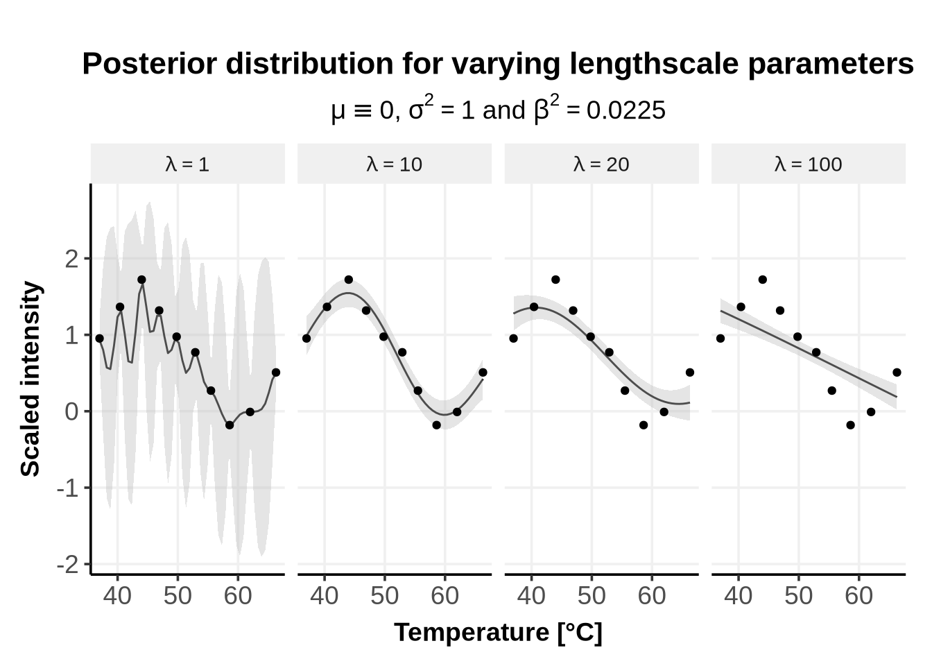

Figure 1: The effect of varying the lengthscale parameter.

As can be seen from Figure 1, if the lengthscale is too small (e.g. \(\lambda = 1\)), the predicted mean rapidly oscillate and interpolate all points. If the lengthscale is too large (e.g. \(\lambda = 100\)), the predicted mean is very straight and almost no points are interpolated.

5 The output-scale parameter

The output-scale \(\sigma^2\) describes how far from the GP’s mean \(\mu\) will the predicted mean typically vary.

lambda_vec <- 10     # Lengthscale
sigma_sq_vec <- c( 1e-6,0.01,0.05, 1)   # Output-scale 
beta_sq_vec <- 0.15^2  # Likelihood variance (same as noise level in y_obs)

gp_results_df <- gp_grid_posterior_distri(
  data_obs$x_obs, 
  data_obs$y_obs,
  lambda_vec, 
  sigma_sq_vec,
  beta_sq_vec,
  n_PredictionsPoints=50)

ggplot() +
  geom_line(data = gp_results_df, aes(x = x, y = mean), color = "black") +
  geom_ribbon(data = gp_results_df,
              aes(x = x, ymin = lower, ymax = upper), fill = "grey", alpha = 0.4) +
  geom_point(data = data_obs, aes(x = x_obs, y = y_obs), na.rm = TRUE, color = "black") +
  facet_grid(.~sigma_sq, labeller = label_bquote(cols = sigma^2 == .(sigma_sq)))+
  xlab("Temperature [°C]") +
  ylab("Scaled intensity") +
  ggtitle("Posterior distribution for varying output-scale parameters",
          subtitle = TeX(paste0("$\\mu \\equiv 0$, $\\lambda = $", lambda_vec, " and $\\beta^2 = $", beta_sq_vec )))+
  theme_Publication()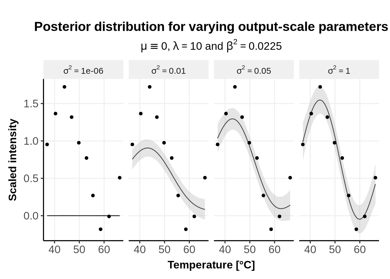

Figure 2: The effect of varying the output-scale parameter.

As can be seen from Figure 2, if the output-scale is close to \(0\) (\(\sigma^2 = 1e^{-6}\)), the posterior mean remains very close to the prior mean, i.e. \(0\) in this case. As the output-scale increases, the posterior mean can go further away from the prior mean. This also explains why the prior mean is often set to \(0\) (see Section 7) instead of specifying a functional form: the kernel alone, and in our case the RBF with output-scale and lengthscale parameters, is enough to accommodate the observations.

6 The noise variance

This variance corresponds to the noise of the error term \(\epsilon\), which we chose to be independent and identically (iid) normally distributed: \[ \epsilon_i \sim \mathcal{N}(0, \beta^2 I)\]

lambda_vec <- 10    # Lengthscale
sigma_sq_vec <- 1  # Output-scale 
beta_sq_vec <- c(0.001, 0.15, 0.5)^2 # Likelihood variance (same as noise level in y_obs)

gp_results_df <- gp_grid_posterior_distri(
  data_obs$x_obs, 
  data_obs$y_obs,
  lambda_vec, 
  sigma_sq_vec,
  beta_sq_vec,
  n_PredictionsPoints=50)

ggplot() +
  geom_line(data = gp_results_df, aes(x = x, y = mean), color = "black") +
  geom_ribbon(data = gp_results_df,
              aes(x = x, ymin = lower, ymax = upper), fill = "grey", alpha = 0.4) +
  geom_point(data = data_obs, aes(x = x_obs, y = y_obs), na.rm = TRUE, color = "black") +
  facet_grid(.~beta_sq, labeller = label_bquote(cols = beta^2 == .(sqrt(beta_sq))^2))+
  xlab("Temperature [°C]") +
  ylab("Scaled intensity") +
    ggtitle("Posterior distribution for varying noise variance parameters",
          subtitle = TeX(paste0("$\\mu \\equiv 0$, $\\lambda = $", lambda_vec, " and $\\sigma^2 = $", sigma_sq_vec )))+
  theme_Publication()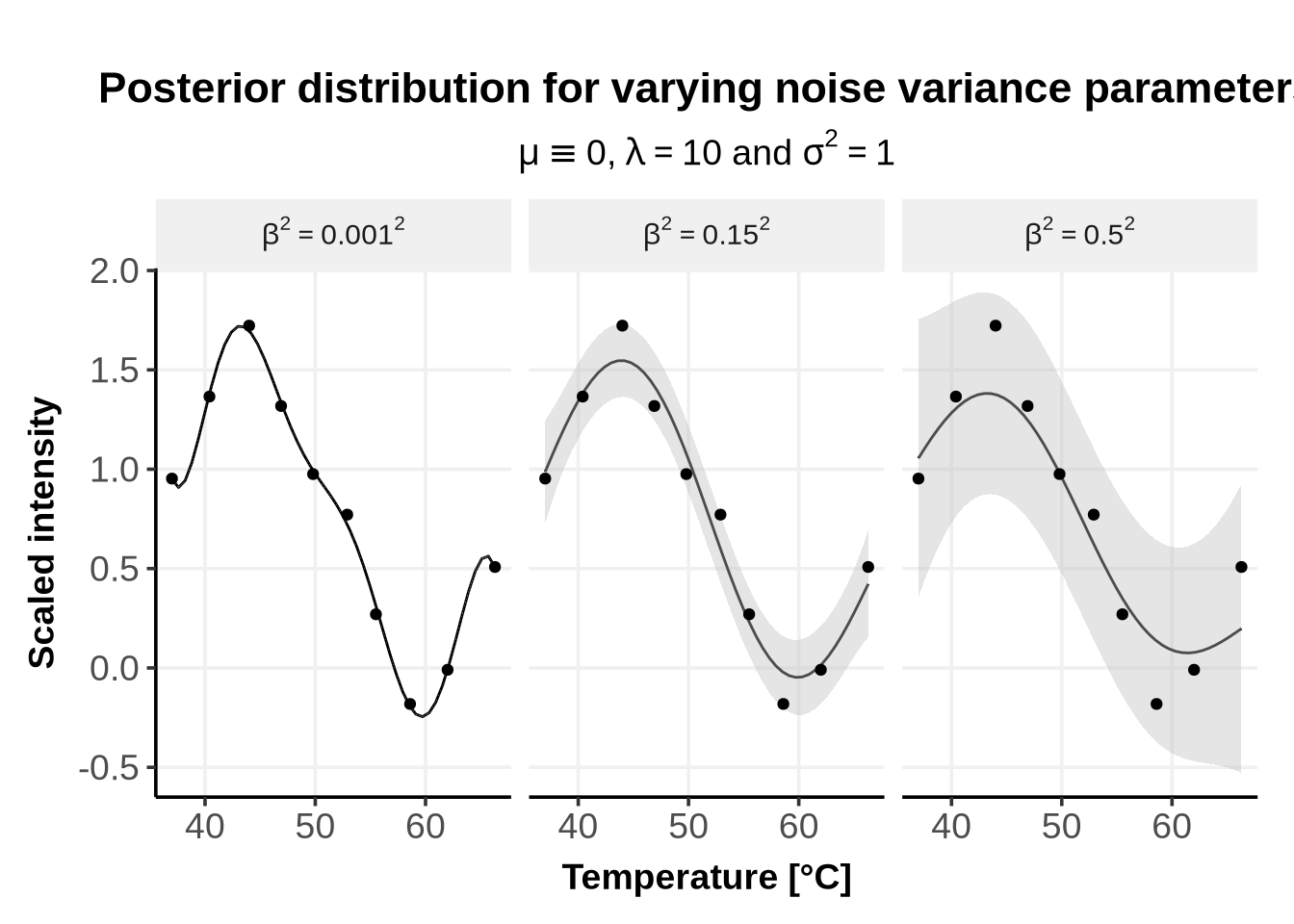

Figure 3: The effect of varying the noise variance parameter.

As can be seen from Figure 3, when the noise variance parameter is extremely small, the model interprets this as “absence of noise”, and the RBF kernel will accomodate almost perfectly all points: this is called over-fitting. On the other hand, if the noise variance parameter is very large, the model interprets this as “the data are very noisy”, and the confidence region becomes vers large, as the fit is less certain.

7 The mean of the GP prior

The mean of a GP prior \(\mu\) is a function. It is generally set to be constantly \(0\), unless strong prior knowledge favor the use of a specific function or value for \(\mu\).

In the current implementation of GPMelt, \(\mu\) can be set to \(0\) or to a constant value \(C\).

Note: all the results of the paper (Le Sueur, Rattray, and Savitski (2024)) are obtained by defining \(\mu \equiv 0\).

lambda_vec <- 10
sigma_sq_vec <- 1.0
beta_sq_vec <- 0.15^2

mean_func_list <- list(
  function(x) 0,                  # Zero mean
  function(x) 6,                  # constant mean
  function(x) 0.5 * x,            # Linear mean
  #function(x) 0.1 * x^2 ,          # Quadratic mean
  function(x) sin(x)           # sin mean
) 

gp_results_df <- gp_grid_posterior_distri(
  data_obs$x_obs, 
  data_obs$y_obs,
  lambda_vec, 
  sigma_sq_vec,
  beta_sq_vec,
  mean_func_list,
  n_PredictionsPoints=50)

mean_func_labels <- c(
  "1" = "Zero mean",          # Zero mean
  "2" = "Constant mean",      # Constant mean
  "3" = "Linear mean",       # Linear mean
  "4" = "Sin mean"         # Sine mean
)

# Custom labeller for mean functions using label_parsed
mean_func_labeller <- labeller(prior_mean_func = mean_func_labels)

# Plot with custom labeller and label_parsed
ggplot() +
  geom_line(data = gp_results_df, aes(x = x, y = mean), color = "black") +
  geom_ribbon(data = gp_results_df,
              aes(x = x, ymin = lower, ymax = upper), fill = "grey", alpha = 0.4) +
  geom_point(data = data_obs, aes(x = x_obs, y = y_obs), na.rm = TRUE, color = "black") +
  facet_grid(.~prior_mean_func, labeller = mean_func_labeller)+
  theme_Publication() +
  xlab("Temperature [°C]") +
  ylab("Scaled intensity") +
  ggtitle("Posterior distribution for different mean functions",
          subtitle = TeX(paste0("$\\lambda = $", lambda_vec, " ,$\\sigma^2 = $", sigma_sq_vec, " and $\\beta^2 = $", beta_sq_vec )))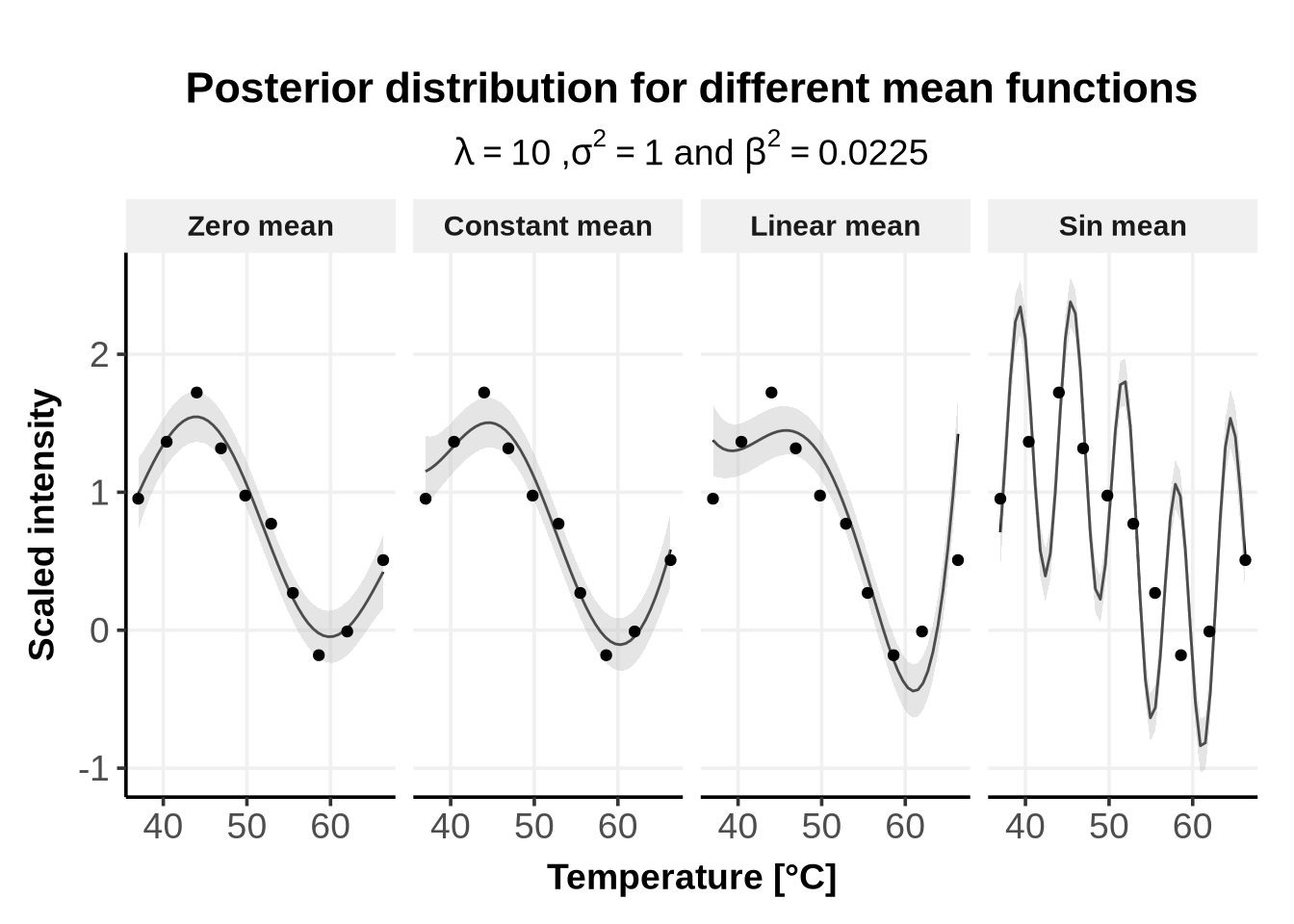

Figure 4: The effect of varying the mean function

In Figure 4 we used the following mean functions:

• Zero mean : \(\mu \equiv 0\),
• Constant mean: \(\mu \equiv 6\),
• Linear mean: \(\mu(t) = 0.5 * t\)
• Sin mean: \(\mu(t) = sin(t)\)

8 Varying the number of test points

Finally, we show the impact of varying the parameter n_PredictionsPoints which defines the number of test points \(X^* =[x_1^*, \cdots, x_{N_{pred}}^*]\).

This parameter is not a GP hyper-parameter, but smoothly fits here.

# Define a vector of different n_PredictionsPoints values
n_PredictionsPoints_values <- c(5, 10, 20, 50)  # Different numbers of prediction points

# Initialize an empty list to store the results
results_list <- list()

# Parameters (keep these the same)
X_obs <- data_obs$x_obs
y_obs <- data_obs$y_obs
lambda <- 10
sigma_sq <- 1.0
beta_sq <- 0.15^2
prior_mean_func <- function(x) 0  # Zero mean

# Loop over different values of n_PredictionsPoints
for (n_points in n_PredictionsPoints_values) {
  
  # Run GP posterior distribution for the current n_PredictionsPoints
  result <- gp_posterior_distri(X_obs, y_obs, lambda, sigma_sq, beta_sq,  prior_mean_func, n_PredictionsPoints = n_points)
  
  # Store the result in a list, including n_PredictionsPoints
  results_list[[as.character(n_points)]] <- data.frame(
    x = result$X_test,
    mean = result$mean,
    lower = result$lower,
    upper = result$upper,
    n_PredictionsPoints = n_points
  )
}

# Combine all results into a single data frame
gp_results_df <- do.call(rbind, results_list)

# Plot the GP posterior for different values of n_PredictionsPoints
ggplot() +
  geom_line(data = gp_results_df, aes(x = x, y = mean), color = "black") +
  geom_ribbon(data = gp_results_df,
              aes(x = x, ymin = lower, ymax = upper), fill = "grey", alpha = 0.4) +
  geom_point(data = gp_results_df, aes(x = x, y = mean , shape = "4"), color = "black") +
  geom_point(data = data_obs, aes(x = x_obs, y = y_obs, shape = "16"), na.rm = TRUE, color = "black") +
  facet_grid(.~n_PredictionsPoints, labeller = label_bquote(cols = N_pred == .(n_PredictionsPoints)))+
  scale_shape_manual(name = "", 
                     values = c("16"=16, 
                                "4"=4),
                     labels = c("16"="training points", 
                                "4"="testing points")
                     )+
  theme_Publication() +
  xlab("Temperature [°C]") +
  ylab("Scaled intensity") +
  ggtitle("Posterior distribution for different number of test points",
          subtitle = TeX(paste0("$\\mu \\equiv 0$, $\\lambda = $", lambda_vec, " ,$\\sigma^2 = $", sigma_sq_vec, " and $\\beta^2 = $", beta_sq_vec )))
  #theme(legend.text = element_blank())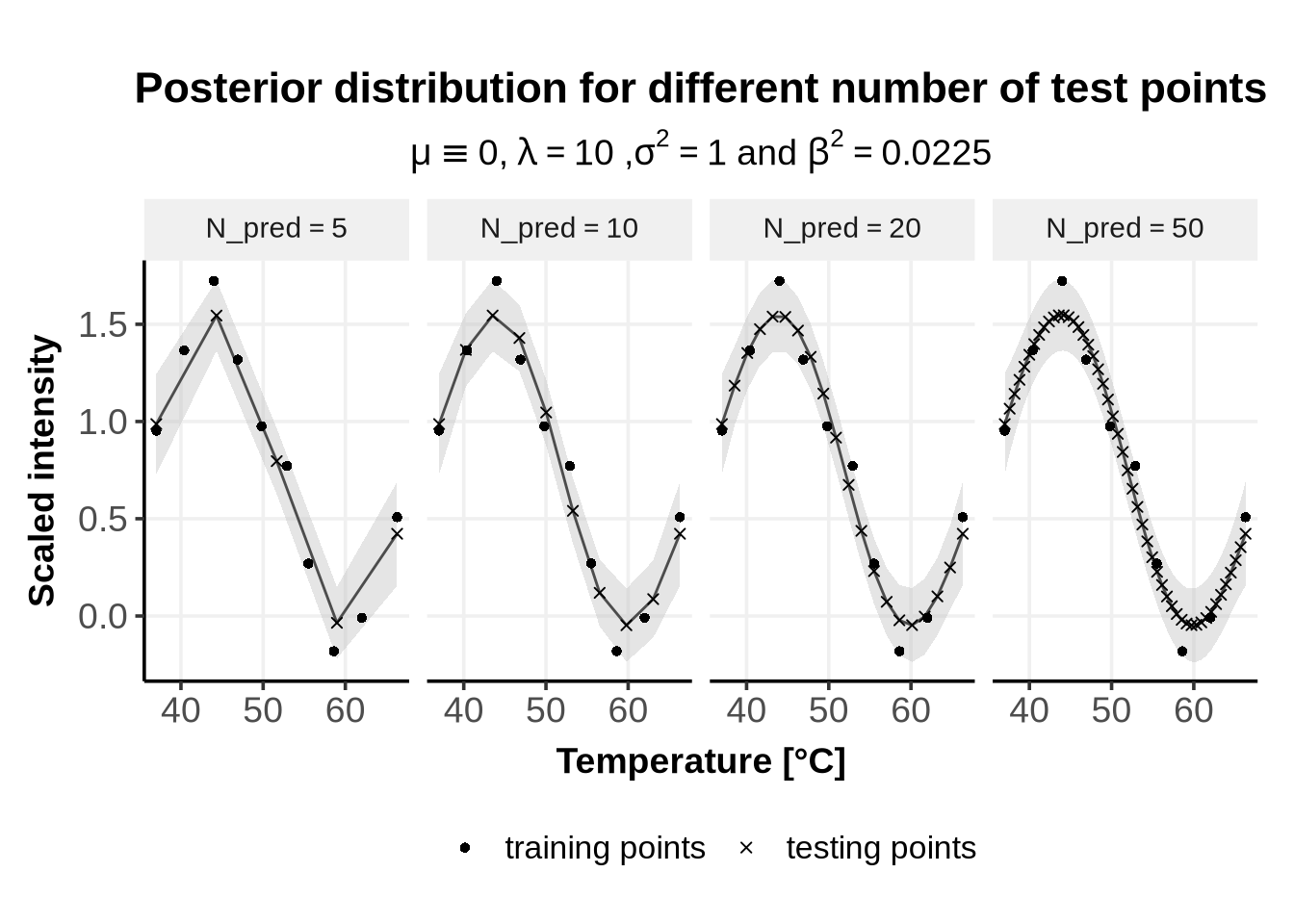

Figure 5: The effect of varying the number of test points

As can be seen from Figure 5, the number of test points influences the smoothness of the prediction. Above n_PredictionsPoints \(= 50\), visual differences are minimal, but greater precision may be necessary depending on individual needs—for instance, when estimating the effect size (explained here, section 5).

9 Session Info

sessionInfo()

R version 4.4.1 (2024-06-14)
Platform: x86_64-conda-linux-gnu
Running under: Debian GNU/Linux 12 (bookworm)

Matrix products: default
BLAS/LAPACK: /opt/conda/lib/libopenblasp-r0.3.27.so;  LAPACK version 3.12.0

locale:
 [1] LC_CTYPE=C.UTF-8       LC_NUMERIC=C           LC_TIME=C.UTF-8       
 [4] LC_COLLATE=C.UTF-8     LC_MONETARY=C.UTF-8    LC_MESSAGES=C.UTF-8   
 [7] LC_PAPER=C.UTF-8       LC_NAME=C              LC_ADDRESS=C          
[10] LC_TELEPHONE=C         LC_MEASUREMENT=C.UTF-8 LC_IDENTIFICATION=C   

time zone: Etc/UTC
tzcode source: system (glibc)

attached base packages:
[1] stats     graphics  grDevices utils     datasets  methods   base     

other attached packages:
[1] latex2exp_0.9.6 ggplot2_3.5.1  

loaded via a namespace (and not attached):
 [1] vctrs_0.6.5       cli_3.6.3         knitr_1.48        rlang_1.1.4      
 [5] xfun_0.48         stringi_1.8.4     generics_0.1.3    jsonlite_1.8.9   
 [9] labeling_0.4.3    glue_1.8.0        colorspace_2.1-1  htmltools_0.5.8.1
[13] scales_1.3.0      fansi_1.0.6       rmarkdown_2.28    grid_4.4.1       
[17] evaluate_1.0.1    munsell_0.5.1     tibble_3.2.1      fastmap_1.2.0    
[21] yaml_2.3.10       lifecycle_1.0.4   stringr_1.5.1     compiler_4.4.1   
[25] dplyr_1.1.4       htmlwidgets_1.6.4 pkgconfig_2.0.3   farver_2.1.2     
[29] digest_0.6.37     R6_2.5.1          tidyselect_1.2.1  utf8_1.2.4       
[33] pillar_1.9.0      magrittr_2.0.3    withr_3.0.1       tools_4.4.1      
[37] gtable_0.3.5     

References

Le Sueur, Cecile, Magnus Rattray, and Mikhail Savitski. 2024. “GPMelt: A Hierarchical Gaussian Process Framework to Explore the Dark Meltome of Thermal Proteome Profiling Experiments.” PLOS Computational Biology 20 (9): e1011632.

Footnotes

1. In GPMelt, all kernels we use are called Radial Basis Function (RBF) kernels, also known as squared-exponential kernels. These kernels are defined by: \[ k(t, t') = \sigma^2 \cdot \exp \left(- \frac{||t -t'||^2}{2\lambda^2}\right) \] We chose this type of kernel because they generate smooth (infinitely differentiable) curves, have only two parameters and are widely used.