Linking hierarchical models to multi-task implementation
1 Conceptual introduction
We begin by introducing a fundamental principle shared by hierarchical models and multi-task learning approaches, using a simple metaphor.
Imagine you’ve just started your PhD, and quickly realise that \(10000\) qualities are expected of you: not only should you be a passionate and dedicated scientist, but also an eloquent linguist, a talented designer of scientific illustrations, a champion of sport and well-being, and a graceful networker.
Like me, you might be feeling a bit overwhelmed:
2 Multi-task learning
Multi-task learning is a field of Machine Learning that aims to share information among related tasks to improve individual task learning and predictions, compared to learning each task independently (Bonilla, Chai, and Williams 2007).
Similarly, the three-level hierarchical model visualised in this Video helps to improve the modeling of each replicate in each condition by sharing information between all replicates across all conditions for each protein.
A task in the multi-task learning framework corresponds to a replicate in our hierarchical model framework.
3 Task similarity matrix
Without delving into mathematical details, we simply need to understand what a task similarity matrix is, and how to define it in the context of our hierarchical models.
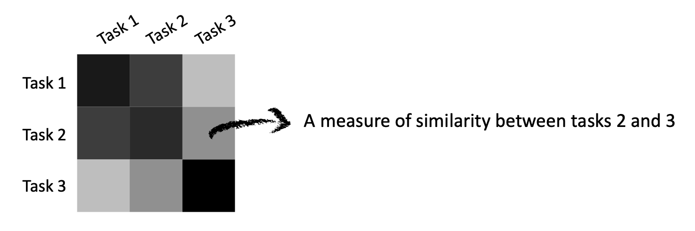
A task similarity matrix can be seen as a lookup table containing a measure of similarity between any two tasks (or replicates in our setting).
This matrix doesn’t need to be fully filled with values. Instead, in our case, these matrices will mostly be sparse (i.e., containing many \(0\) entries).
4 Breaking down similarities into interpretable matrices
We use task similarity matrices to translate our prior beliefs about task similarities into mathematical terms. Fortunately, you don’t need to write any equations here - just defining the task similarity matrix structure is enough, as GPMelt handles the rest ;)
We will proceed by breaking down task similarities, considering each level of the hierarchy. This approach results in simple and interpretable task similarity matrices. Note that this means defining as many task similarity matrices as there are levels in the hierarchy.
With Video 2, we illustrate how to proceed using the example presented in this earlier video. Detailed explanations are given in the sections after the video.
4.1 Bottom level of the hierarchy
We begin with the lowest level of the hierarchy, i.e. the leaves, also described earlier as the replicate level. At this level, we do not assume any similarities across tasks yet. Therefore, all entries of the task similarity matrix, except the diagonal, will be set to \(0\).
Next, we want to model the fact that points within a replicate are correlated, so we fill in the diagonal of the matrix. To fill these entries simply means telling GPMelt to estimate a value for them.
You have two choices for these values.
The simplest option is to estimate a single value for all entries of the diagonal. This means that we believe that all replicates have the same level of correlation between their observations - in other words, all replicates are approximately equally noisy.
The second option is to estimate a different value for each diagonal entry, where each value indicates how noisy a specific replicate is.
Why does this matter? The value estimated for each task is called an output-scale. We consider our hierarchical example with three levels, the second level being the conditions and the first the protein. The output-scale associated to a replicate measures how much the curve for that replicate deviates from the curve for the condition it belongs to. If a replicate is noisy or present an outlier observation or a outlier shape, the output-scale will be large, indicating a significant deviation from the condition curve.
You don’t need to define the output-scale values yourself—they will be estimated. However, you do need to choose whether to estimate a single value for all replicates or different values for each replicate.
How to decide? We recommend two ways:
- If you already noticed that the replicates are noisy, we recommend estimating a different value for each replicate.
- If you are unsure, we suggest starting with the simplest model (a single value for all replicates) and then trying different model specifications. Examining a few fits will help you decide whether constraining the output-scale to one value is too restrictive (for example, if the fits seem a bit off).
4.2 Second level of the hierarchy
While users have the option to choose between unique or multiple output-scale values for the bottom level, this is not the case for the second and first levels of the hierarchy.
Important:
- Due to the requirements of the hypothesis testing framework, the first two levels of the hierarchy are constrained to have only one output-scale estimated per level.
- Any additional level in the hierarchy can have free (i.e. one per task) or fixed (i.e. the same for all tasks) output-scales.
The condition-level task similarity matrix doesn’t need to be specified by the user, but we still explain below how it should look so the user can check the validity of the model specification when reviewing the plots produced by GPMelt (see here, section 7).
This level translates our prior belief that replicates within a condition are expected to show similar melting behaviors, hence individual replicates are grouped into a bigger group - the condition. Considering the second level of the hierarchy, these groups can now be seen as tasks. Because we share the output-scales for all conditions, this means that we model each condition as deviating by roughly the same amount from the protein-wise melting curve (level above).
Continuing with our TPP-TR example, conditions are represented by blocks on the diagonal of the matrix, as illustrated in Video 2.
4.3 Top level of the hierarchy
Finally, the top level of the hierarchy reflects our belief that, if the conditions have no effect on the protein’s melting curve, then all replicates across all conditions should exhibit similar behaviour. This is represented by a task similarity matrix where all entries are non-zero. Additionally, we impose the constraint that all entries in this matrix are the same.
4.4 Complete task similarity matrix
The complete task similarity matrix is simply (in this case) the sum of all level-associated task similarity matrices in this case.
As we will discuss here, you can relax certain constraints to make the model more or less complex if necessary.
5 Why break down the task similarity matrix?
Why did we decompose the task similarity matrix into three sub-matrices instead of directly learning a full task similarity matrix with specific similarities for each pair of replicates?
This could have been done, but it wouldn’t have captured our assumptions about how replicates relate to one another. The model would have been less interpretable and much more complex to learn, especially with a large number of replicates and conditions.
In GPMelt, we construct a model that captures a wealth of information about replicate similarity and the presence of possible outliers while only estimating a limited number of output-scales: one for the first level, one for the second level, and at most one per replicate for the bottom level. This is far fewer than estimating an output-scale for every pair of replicates.
From a theoretical perspective, decomposing the task similarity matrix creates a clear link between the hierarchical model (the mathematical model) and the multi-task learning approach (the model implementation).
Finally, this approach makes it easier to extend the GPMelt model to more complex settings. Once the principle of task similarity matrix decomposition is understood, you can adapt this model to any experimental protocol, even in much more complicated scenarios!