GPMelt workflow and Nextflow encapsulation
We now describe the general GPMelt workflow as it is defined in the form of a Nextflow pipeline.
1 Principle of the workflow
The Nextflow pipeline is composed of four blocks.
INPUT_FORMATTING(with or without IDs subset)RUN_GPMELT_IN_BATCHGATHER_AND_SAVE_RESULTSCOMPUTE_GPMELT_STATISTICS
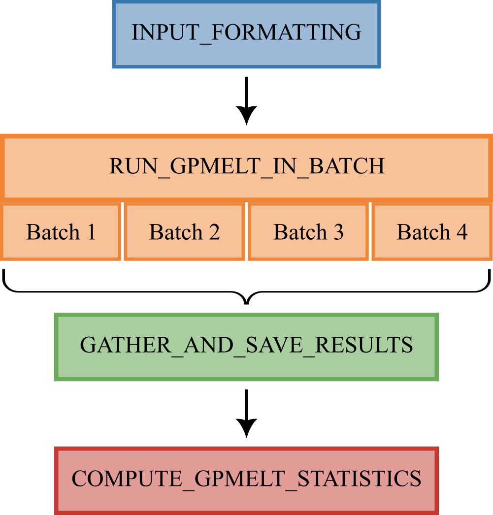
2 INPUT_FORMATTING
In this block, the following steps are done:
- read the
parameters.txtfile in a parameter dictionary. - read the dataset saved as
dataForGPMelt.csvin the tutorial. - check the validity of the model & data columns. For example, if a four-level HGP model is selected but that one of the following variable is missing (
Level_1,Level_2,Level_3,Level_4) then the code stops and report an error message. - scale the data if required & save the scaled data as
data_with_scalingFactors.csvin the final directory. - subset the columns required for GPMelt, sort the variables of the dataset & subset the IDs (if required).
- read the number of samples per IDs using
NumberSamples_perID.csv, - combine the IDs in batches for parallel computing (the size of the batch is defined by the variable
number_IDs_per_jobsinuser_params.config, see here) and save one.pklfile for each group (containing the data for these IDs, the number of samples to draw for each of these IDs for the null distribution approximation and a copy of the parameter dictionary). - output the list of
.pklfiles on which GPMelt should be run, which is saved on the temporary working directory of the Nextflow workflow
3 RUN_GPMELT_IN_BATCH
Steps 1 to 8 described in Section 6 are performed in this part of the workflow. It consists in fitting the model, computing the null distribution approximation and evaluating the statistic \(\Lambda\).
In the current implementation, we propose to group IDs in batches. Inside a batch of IDs, steps 1 to 8 are run for each ID sequentially. However, Nextflow parallelise over these batches of IDs.
Note: we choose to perform the fitting for each ID independently, thus we can parallelise over IDs. In practice, the code is parallelising over Level_1, which can correspond to something else than IDs.
4 GATHER_AND_SAVE_RESULTS
This step gathers the results of all the batches, and save the plots and results files.
5 COMPUTE_GPMELT_STATISTICS
This step performs the p-values computation (step 10 described in Section 6) according to the null distribution approximation method selected by the user (ID-wise or dataset-wise).
6 Algorithmic steps of GPMelt (for advanced users)
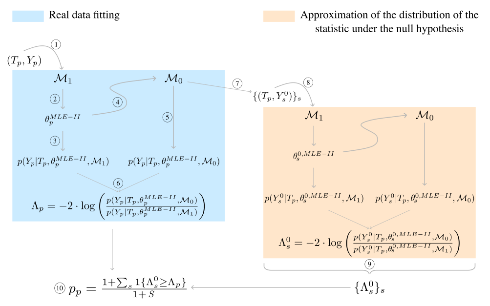
- The procedure starts by feeding the observed data \((T_p, Y_p)\) of protein \(p\) to the full model \(\mathcal{M}_1\) for fitting via type II MLE.
- The obtained parameters estimates are given by \(\theta_p^{MLE-II}\).
- The parameters estimates are used to compute the log marginal likelihood of the observations for this model \(\log \, p(Y_p | T_p, \theta_p^{MLE-II},\mathcal{M}_1)\).
- The parameters estimates are then plugged into the joint model \(\mathcal{M}_0\) which only differs from the full model \(\mathcal{M}_1\) by a change in the covariance matrix structure.
- The log marginal likelihood of the observations for this joint model \(\log \, p(Y_p | T_p, \theta_p^{MLE-II},\mathcal{M}_0)\) are computed.
- The statistic \(\Lambda_p\) is defined as the ratio of the previously computed log marginal likelihood.
- The joint model \(\mathcal{M}_0\) with plugged in parameters estimates \(\theta_p^{MLE-II}\) is used to draw \(S\) samples \(\{(T_p, Y_s^0)\}_s\) from the null hypothesis. It can be noticed that the temperatures \(T_p\) are the same as for the real data.
- Each sample \((T_p, Y_s^0)\) then goes to the same steps as described before. Fitting the model \(\mathcal{M}_1\) to this sample provides the parameters’ type II MLE \(\theta_s^{0,MLE-II}\). \(\theta_s^{0,MLE-II}\) is used to evaluate the log marginal likelihood of the sample under \(\mathcal{M}_1\) and \(\mathcal{M}_0\), given that the parameters of \(\mathcal{M}_0\) have been fixed to \(\theta_s^{0,MLE-II}\). Finally, the statistic \(\Lambda_s^0\) is computed for this sample. \(\Lambda_s^0\) represents a value of the statistic under the null hypothesis.
- The statistics of all samples \(\{\Lambda_s^0\}_s\) are combined to form the approximation of the distribution of the statistic \(\Lambda\) under the null.
- The p-value associated with \(\Lambda_p\) is computed from \(\{\Lambda_s^0\}_s\) similarly as a permutation p-value.
Note: depicted here is the protein-wise null distribution approximation (methods B and D of Table E in S1 File). If the null distribution approximation is obtained by combining samples from all proteins of the dataset (i.e. dataset-wise methods A and C of Table E in S1 File), then the set \(\{\Lambda_{ps}^0\}_s\) of values of the statistic under the null obtained for protein \(p\) is combined with the sets obtained for all other proteins. The p-value (step 10) is computed using this combined set \(\{\Lambda_{ps}^0\}_{p, s}\) instead of \(\{\Lambda_s^0\}_s\). Similarly, for the group-wise method E of Table E in S1 File, the p-value of a protein in a group is computed using the combined set \(\{\Lambda_{ps}^0\}_{p, s}\) over all proteins \(p\) belonging to this group.